Introduction
SRTF stands for Shortest Remaining Time First. It is also known as preemptive SJF because it allows a shorter newly arrived process to interrupt the currently running process.
The key idea is remaining time. Instead of comparing only original burst time, SRTF compares how much CPU time each available process still needs.
Core Rule of SRTF Scheduling
In SRTF scheduling, the operating system always selects the available process with the least remaining CPU time. If a new process arrives with a shorter remaining time than the currently running process, the current process is preempted.
This makes SRTF different from non-preemptive SJF. In SJF, a running process continues once selected. In SRTF, the scheduler can change its decision whenever a better short job becomes available.
SRTF is more dynamic than non-preemptive SJF, so it needs a few extra conditions:
Preemption: The operating system must be able to interrupt a running process.
Context switching: The OS must save one process state and load another process state.
Remaining-time estimate: The scheduler needs to know or predict how much CPU time each process still requires.
Because of these requirements, SRTF can give better average performance, but it also creates more scheduling overhead.
SRTF Scheduling Example
Consider five processes with arrival time and burst time:
Process | Arrival Time | Burst Time |
|---|---|---|
P1 | 0 | 8 |
P2 | 1 | 4 |
P3 | 2 | 9 |
P4 | 3 | 5 |
P5 | 7 | 2 |
The compact scheduling flow is:
Time 0: Only
P1has arrived, soP1starts.Time 1:
P2arrives with burst time4, whileP1has7units remaining, soP2preemptsP1.Time 5:
P2completes, andP4has the shortest remaining time among available processes.Time 7:
P5arrives with burst time2, whileP4has3units remaining, soP5preemptsP4.After P5:
P4resumes, thenP1, and finallyP3.
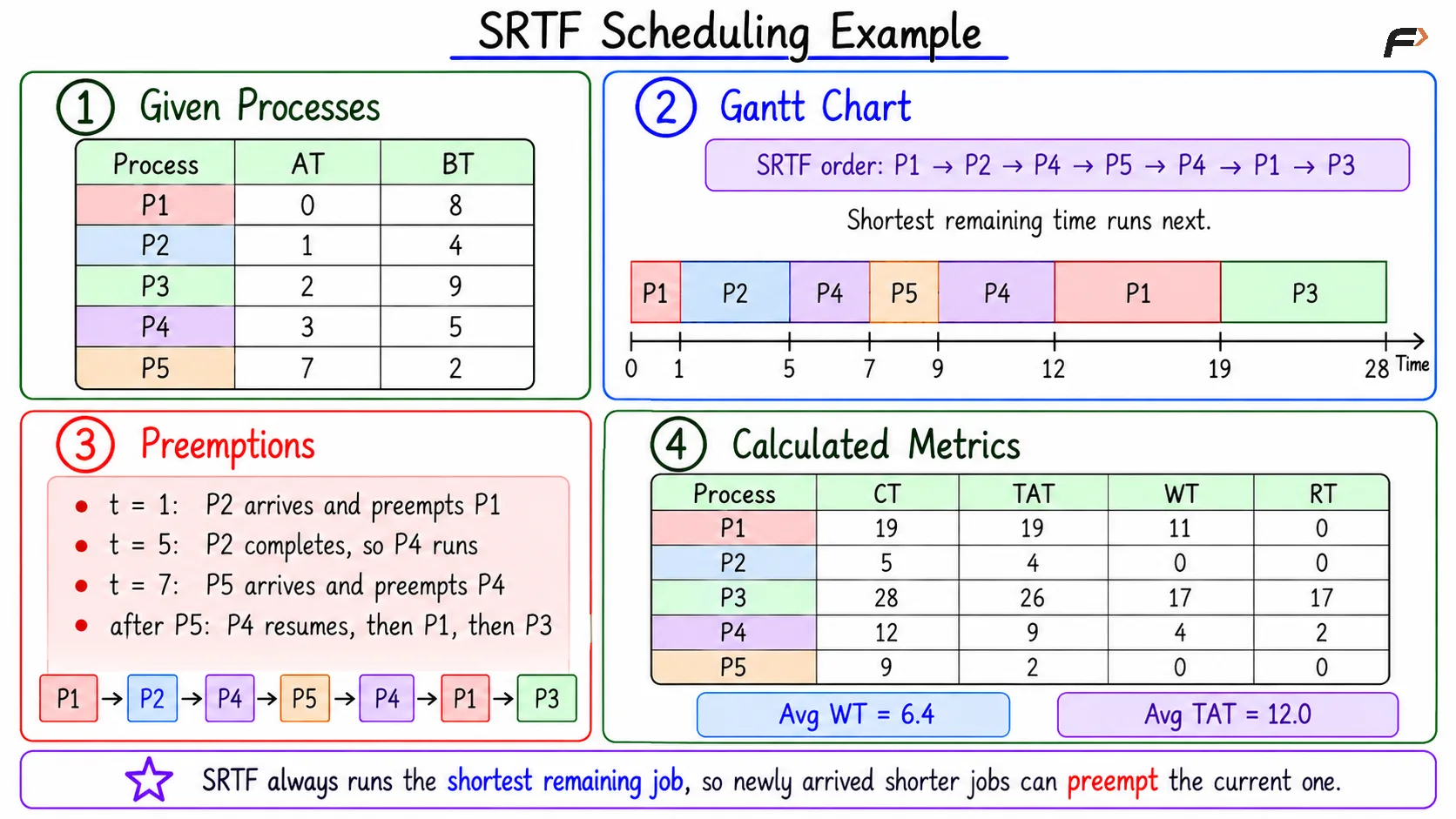
SRTF Scheduling Example
Process | CPU Time Interval |
|---|---|
P1 | 0 to 1 |
P2 | 1 to 5 |
P4 | 5 to 7 |
P5 | 7 to 9 |
P4 | 9 to 12 |
P1 | 12 to 19 |
P3 | 19 to 28 |
Metric Calculation
The main formulas are:
CT: finish time of the process
TAT:
CT - ATWT:
TAT - BTRT:
first start time - AT
Process | CT | TAT | WT | RT |
|---|---|---|---|---|
P1 | 19 | 19 | 11 | 0 |
P2 | 5 | 4 | 0 | 0 |
P3 | 28 | 26 | 17 | 17 |
P4 | 12 | 9 | 4 | 2 |
P5 | 9 | 2 | 0 | 0 |
Average TAT = 12.0, average WT = 6.4, and average RT = 3.8.
Why Waiting Time and Response Time Differ
In SRTF, a process may start once, get preempted, and then wait again before completing. Because of this, waiting time and response time are not always the same.
For example, P1 starts immediately at time 0, so its response time is 0. But after being preempted at time 1, it waits until time 12, so its total waiting time becomes much larger.
Strengths and Weaknesses of SRTF
Strengths | Weaknesses |
|---|---|
Gives very good average waiting time | Needs remaining-time estimation |
Improves average turnaround time | Long processes may starve |
Quickly completes short jobs | More context switching overhead |
Shows the benefit of preemption | Hard to apply exactly in real systems |
Summary
SRTF scheduling runs the process with the least remaining CPU time. It is preemptive, so a newly arrived short process can interrupt the currently running process.
It usually improves average waiting time and turnaround time, especially for short jobs. However, it needs remaining-time prediction, increases context-switching overhead, and may cause starvation for long processes.
Be the first to add a comment.