Introduction
Multilevel Queue Scheduling, or MLQ, is used when one ready queue is not enough for all process categories. Instead of treating every process the same way, the scheduler separates them into fixed queues.
This is useful because system tasks, interactive tasks, and batch tasks often need different scheduling behavior. Some work needs fast response, while some background work can wait longer.
Core Idea of MLQ Scheduling
Different process classes may have different importance and response needs. MLQ helps the operating system organize these classes instead of mixing all ready processes into one queue.
Common queue categories include System tasks, Interactive tasks and Batch tasks. Each process is assigned to one queue when it enters the system.
Each queue can have its own priority, scheduling algorithm, and CPU share. For example, a system queue may have strict priority, while an interactive queue may use Round Robin and a batch queue may use FCFS.
MLQ Scheduling Example
Consider three fixed queues:
Queue | Process Class | Priority |
|---|---|---|
Q0 | System | Highest |
Q1 | Interactive | Medium |
Q2 | Batch | Lowest |
Inside each queue, FCFS is used. Higher queues can preempt lower queues, and processes do not move between queues.
Given processes:
Process | Arrival Time | Burst Time | Queue |
|---|---|---|---|
P1 | 0 | 8 | Batch |
P2 | 1 | 4 | Interactive |
P3 | 2 | 9 | Batch |
P4 | 3 | 5 | Interactive |
P5 | 7 | 2 | System |
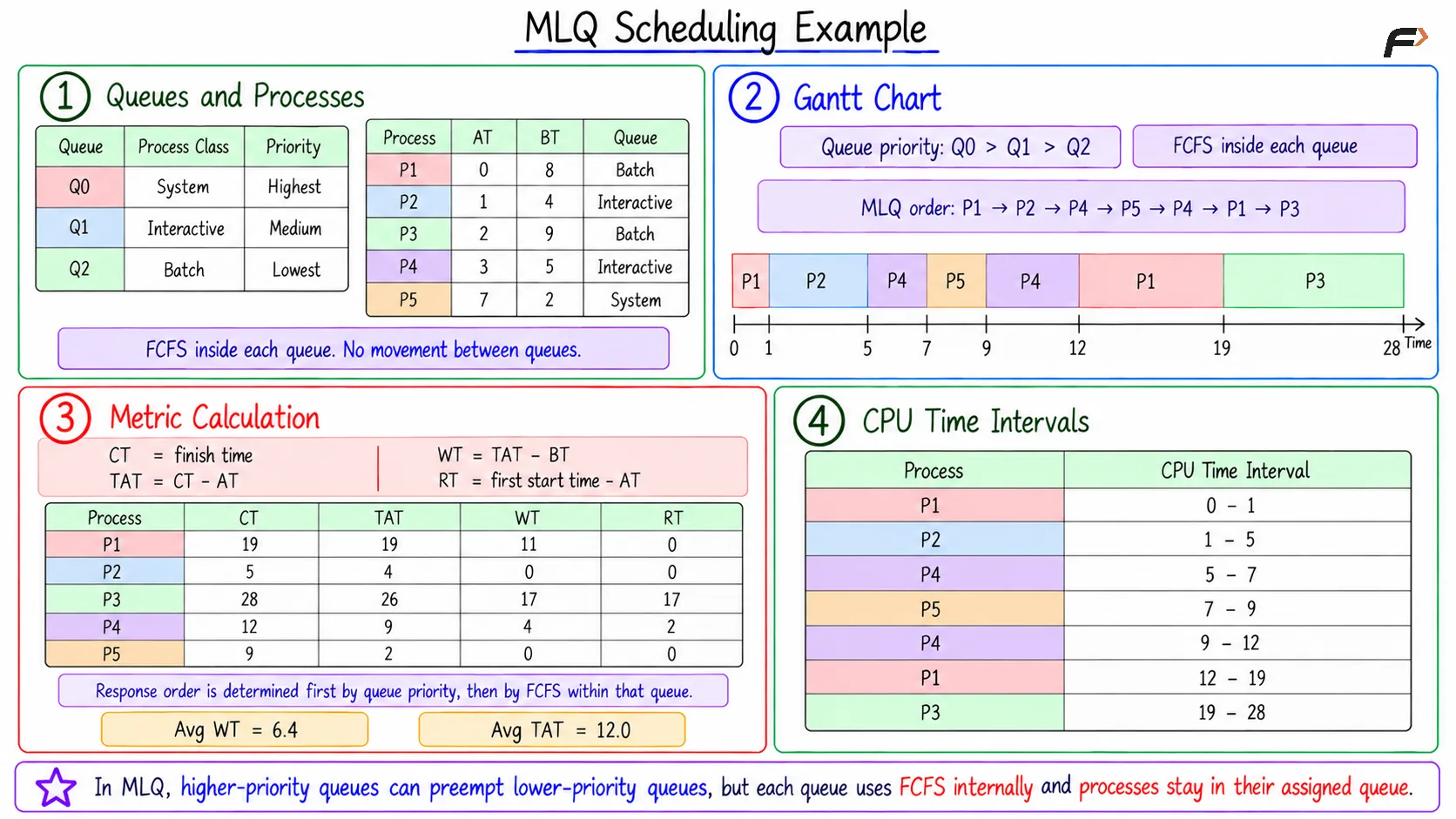
MLQ Scheduling Example
The compact scheduling flow is:
At time
0, onlyP1is available, soP1starts inQ2.At time
1,P2arrives inQ1and preemptsP1.P3arrives inQ2, but it cannot preemptP2.P4arrives inQ1, but FCFS insideQ1keepsP2running.At time
5,P2finishes andP4starts.At time
7,P5arrives inQ0and preemptsP4.After
P5,P4resumes, thenP1, and finallyP3.
Process | CPU Time Interval |
|---|---|
P1 | 0 to 1 |
P2 | 1 to 5 |
P4 | 5 to 7 |
P5 | 7 to 9 |
P4 | 9 to 12 |
P1 | 12 to 19 |
P3 | 19 to 28 |
Metric Calculation
The main formulas are:
CT: time when the process finishes
TAT:
CT - ATWT:
TAT - BTRT:
first CPU start time - AT
Process | CT | TAT | WT | RT |
|---|---|---|---|---|
P1 | 19 | 19 | 11 | 0 |
P2 | 5 | 4 | 0 | 0 |
P3 | 28 | 26 | 17 | 17 |
P4 | 12 | 9 | 4 | 2 |
P5 | 9 | 2 | 0 | 0 |
Average TAT = 12.0, average WT = 6.4, and average RT = 3.8.
Strengths and Weaknesses of MLQ
Strengths | Weaknesses |
|---|---|
Separates different workload classes | Fixed queue assignment is rigid |
Allows each queue to use its own scheduling policy | Lower-priority queues may starve |
Protects critical system and interactive tasks | Wrong classification can reduce performance |
Simple to reason about once queues are defined | Does not adapt to behavior changes in basic MLQ |
If a process is placed in the wrong queue, the scheduler does not automatically move it to a better queue in the basic MLQ model. This is one major difference between MLQ and Multilevel Feedback Queue scheduling.
Summary
Multilevel Queue Scheduling divides the ready queue into multiple fixed queues for process classes such as system, interactive, and batch work. The scheduler first chooses the highest non-empty queue, then applies the scheduling policy inside that queue.
MLQ is simple and useful when process categories are clear, but it is rigid because processes do not move between queues. Its main concerns are fixed classification, queue priority design, and starvation prevention for lower-priority queues.
Be the first to add a comment.