Introduction
Multilevel Feedback Queue Scheduling, or MLFQ, is an extension of Multilevel Queue Scheduling. The key difference is feedback.
In MLQ, a process stays in its assigned queue. In MLFQ, processes can move between queues depending on how they behave during execution.
Why MLFQ Scheduling Is Needed
MLQ is rigid because each process remains in the queue where it was first classified. If that classification is wrong, the scheduler does not adapt in the basic MLQ model.
MLFQ solves this by using observed behavior. A process that behaves like an interactive job can stay near the top, while a CPU-heavy process gradually moves to lower-priority queues.
Core Idea of MLFQ
MLFQ uses multiple priority queues. Higher queues have higher priority and usually smaller time quanta, while lower queues have lower priority and may have larger time quanta.
Common rules are:
Higher queues run first: A process in a higher-priority queue is chosen before lower-priority work.
Same queue uses Round Robin: Processes at the same priority level usually share CPU time.
New jobs enter the top queue: New processes are treated optimistically at first.
Full quantum causes demotion: A process that uses its entire time quantum is moved down.
Priority boost prevents starvation: Waiting processes may be moved up after some time.
MLFQ Scheduling Example
Consider five processes:
Process | Arrival Time | Burst Time |
|---|---|---|
P1 | 0 | 9 |
P2 | 1 | 4 |
P3 | 1 | 5 |
P4 | 2 | 4 |
P5 | 3 | 2 |
Queue setup:
Queue | Priority | Policy |
|---|---|---|
Q0 | Highest | Round Robin, quantum = 2 |
Q1 | Medium | Round Robin, quantum = 4 |
Q2 | Lowest | FCFS |
All new jobs enter Q0. Using the full quantum causes demotion. No priority boost is used in this short example.
The compact scheduling flow is:
P1runs from0 to 2inQ0and moves down.P2runs from2 to 4inQ0and moves down.P3runs from4 to 6inQ0and moves down.P4runs from6 to 8inQ0and moves down.P5runs from8 to 10inQ0and finishes.P1runs from10 to 14inQ1and moves down.P2runs from14 to 16inQ1and finishes.P3runs from16 to 19inQ1and finishes.P4runs from19 to 21inQ1and finishes.P1runs from21 to 24inQ2and finishes.
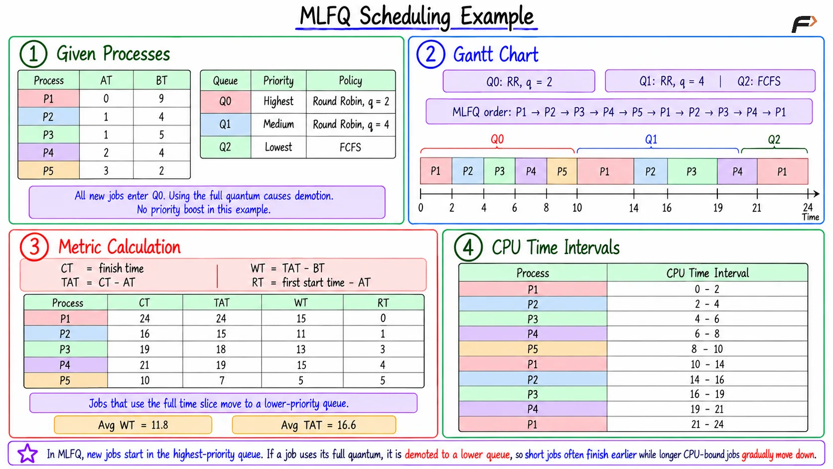
MLFQ Scheduling Example
Process | CPU Time Interval |
|---|---|
P1 | 0 to 2 |
P2 | 2 to 4 |
P3 | 4 to 6 |
P4 | 6 to 8 |
P5 | 8 to 10 |
P1 | 10 to 14 |
P2 | 14 to 16 |
P3 | 16 to 19 |
P4 | 19 to 21 |
P1 | 21 to 24 |
Metric Calculation
The main formulas are:
CT: time when the process finishes
TAT:
CT - ATWT:
TAT - BTRT:
first CPU start time - AT
Process | CT | TAT | WT | RT |
|---|---|---|---|---|
P1 | 24 | 24 | 15 | 0 |
P2 | 16 | 15 | 11 | 1 |
P3 | 19 | 18 | 13 | 3 |
P4 | 21 | 19 | 15 | 4 |
P5 | 10 | 7 | 5 | 5 |
Average TAT = 16.6, average WT = 11.8, and average RT = 2.6.
Strengths and Weaknesses of MLFQ
Strengths | Weaknesses |
|---|---|
Adapts to process behavior | Has many parameters to tune |
Gives good response to short and interactive jobs | Can be more complex to implement |
Does not require exact burst-time knowledge | Can be exploited by processes that game the rules |
Priority boosting helps prevent starvation | Lower queues may starve without boosting |
Summary
MLFQ scheduling uses multiple priority queues and allows processes to move between them. New jobs usually enter the top queue, CPU-heavy jobs move down, and waiting jobs may be boosted up to reduce starvation.
It improves on rigid MLQ by using feedback from process behavior instead of fixed classification alone. Its main challenges are choosing queue levels, time quanta, demotion rules, and boost intervals carefully.
Be the first to add a comment.