Introduction
FCFS stands for First Come, First Served. It is also called FIFO scheduling because processes are executed in the same order in which they arrive.
The rule is simple: the process that arrives first gets the CPU first. FCFS is easy to understand and implement, but it is mainly useful as a basic scheduling algorithm and comparison point.
Core Rule of FCFS Scheduling
In FCFS scheduling, processes are selected from the ready queue according to arrival time. Once a process gets the CPU, the operating system does not forcibly remove it.
This makes FCFS a non-preemptive scheduling algorithm. A running process gives up the CPU only when it finishes, blocks for I/O, or waits for some event.
FCFS has a few simple properties that make it easy to identify:
Non-preemptive: A running process is not interrupted by the scheduler.
FIFO queue based: Processes are arranged according to arrival order.
Low overhead: The scheduler does not need complex decision-making.
Fair by arrival time: The process that arrives earlier gets the CPU earlier.
Fair by arrival time does not always mean fair by user experience. A short process may still wait a long time if it arrives behind a long process.
Convoy Effect in FCFS
The main weakness of FCFS is the convoy effect. This happens when a long CPU-bound process arrives first and holds the CPU while many shorter processes wait behind it.
Because FCFS does not preempt the running process, short jobs cannot move ahead even if they need very little CPU time. This can increase average waiting time and make the system feel slow, especially in mixed workloads with both CPU-bound and I/O-bound processes.
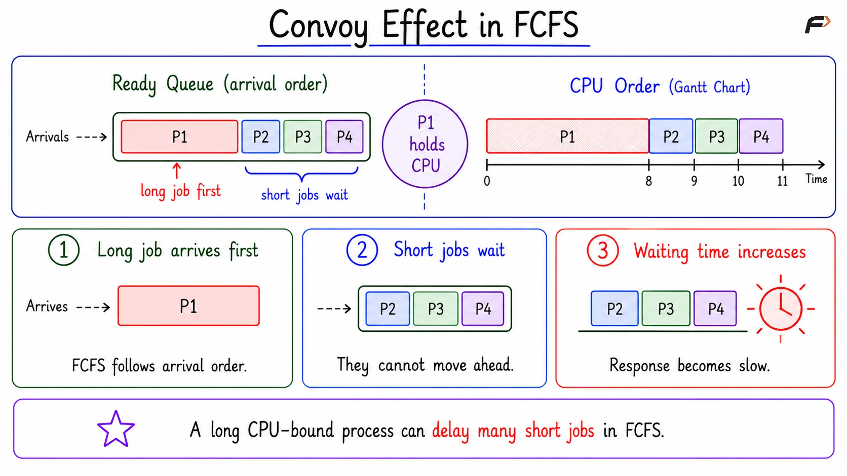
Convoy Effect in FCFS
FCFS Scheduling Example
Consider five processes with arrival time and burst time:
Process | Arrival Time | Burst Time |
|---|---|---|
P1 | 0 | 8 |
P2 | 1 | 4 |
P3 | 2 | 9 |
P4 | 3 | 5 |
P5 | 7 | 2 |
FCFS follows arrival order, so the execution order is P1, P2, P3, P4, P5. Process names alone should not be trusted; arrival time decides the FCFS order.
Process | CPU Time Interval |
|---|---|
P1 | 0 to 8 |
P2 | 8 to 12 |
P3 | 12 to 21 |
P4 | 21 to 26 |
P5 | 26 to 28 |
Metric Calculation
The main formulas are:
CT: finish time of the process
TAT:
CT - ATWT:
TAT - BTRT:
first start time - AT
For example, P2 finishes at time 12. Its arrival time is 1, burst time is 4, and first CPU start time is 8. So, TAT = 12 - 1 = 11, WT = 11 - 4 = 7, and RT = 8 - 1 = 7.
Process | CT | TAT | WT | RT |
|---|---|---|---|---|
P1 | 8 | 8 | 0 | 0 |
P2 | 12 | 11 | 7 | 7 |
P3 | 21 | 19 | 10 | 10 |
P4 | 26 | 23 | 18 | 18 |
P5 | 28 | 21 | 19 | 19 |
Average TAT = 16.4, average WT = 10.8, and average RT = 10.8.
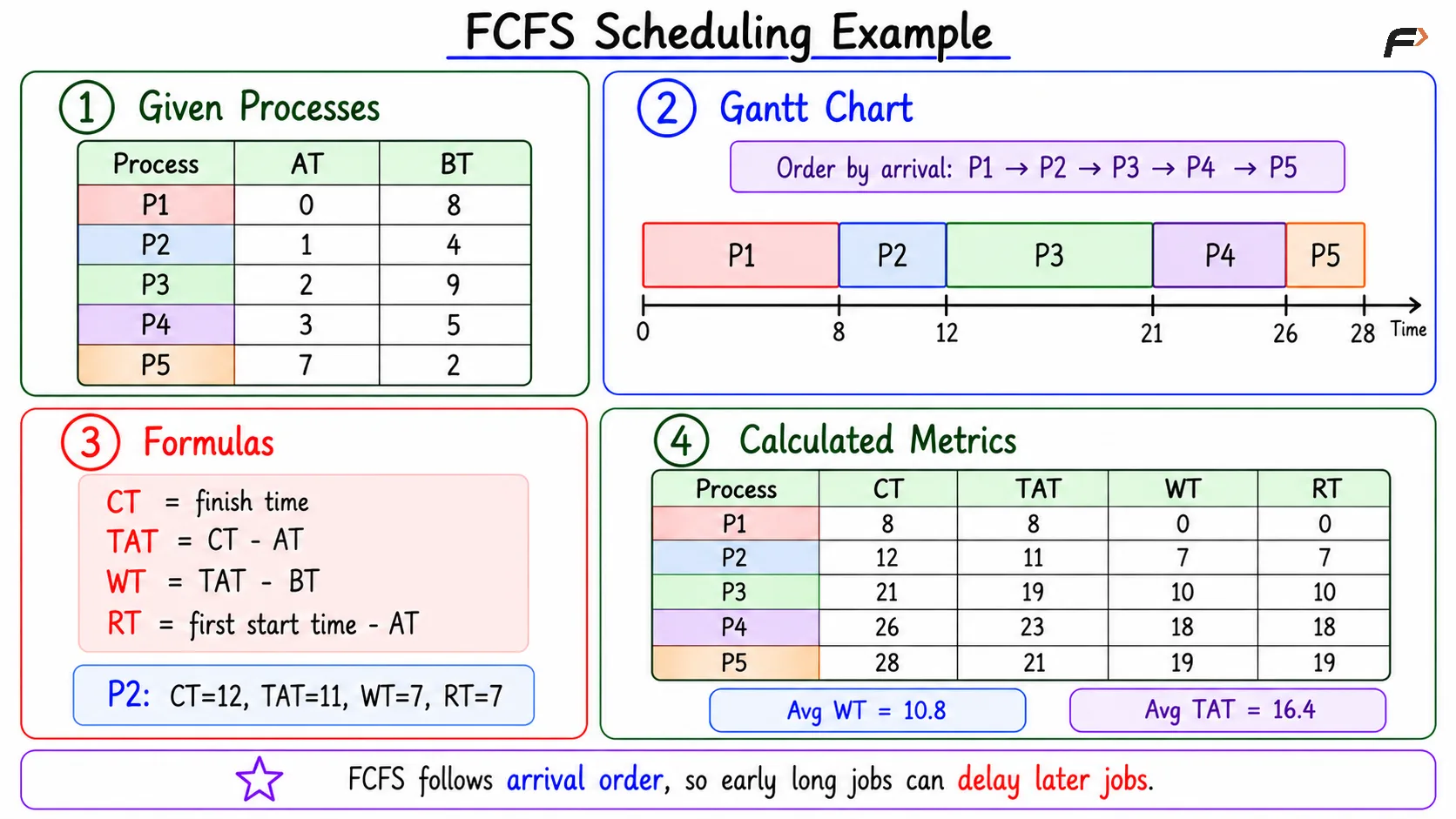
FCFS Scheduling Example
Strengths and Weaknesses of FCFS
Strengths | Weaknesses |
|---|---|
Very easy to understand and implement | Poor response time for short or interactive processes |
Low scheduling overhead | Convoy effect can increase waiting time |
No priority starvation | Not suitable as the main scheduler for modern general-purpose systems |
Summary
FCFS scheduling runs processes in the order they arrive in the ready queue. It is also called FIFO scheduling and is non-preemptive because the running process is not forcibly interrupted.
Its strengths are simplicity, low overhead, and no priority starvation. Its major weakness is the convoy effect, where one long CPU-bound process can delay many shorter processes and increase average waiting time.
Be the first to add a comment.