Introduction
A support dashboard takes several seconds to load a customer’s latest tickets. Another report opens quickly but shows the wrong ticket count. Both need investigation, although the causes may be different.
SQL performance tuning improves how efficiently a query uses time and resources. SQL debugging finds why a query fails, returns unexpected results, or performs unnecessary work. A useful starting point is to establish the expected answer, inspect the query’s execution plan, and measure the effect of a focused change.
Start With a Clear Expected Result
Consider a support application with this tickets table. Each row represents one ticket, ticket_id is its primary key, and customer_id cannot be NULL.
ticket_id | customer_id | opened_at |
|---|---|---|
401 | 7 | 2026-04-10 09:00:00 |
402 | 7 | 2026-04-10 15:30:00 |
403 | 8 | 2026-04-11 10:00:00 |
404 | 7 | 2026-04-12 08:45:00 |
405 | 9 | 2026-04-12 11:00:00 |
We want customer 7's latest two tickets opened from April 10 through April 12. All timestamps in this example use the same reporting time zone.
SELECT ticket_id, opened_atFROM ticketsWHERE customer_id = 7 AND opened_at >= '2026-04-10 00:00:00' AND opened_at < '2026-04-13 00:00:00'ORDER BY opened_at DESC, ticket_id DESCLIMIT 2;Output
ticket_id | opened_at |
|---|---|
404 | 2026-04-12 08:45:00 |
402 | 2026-04-10 15:30:00 |
Three tickets satisfy the filters. Sorting newest first and taking two returns 404 and 402. The additional ordering by ticket_id makes the result deterministic if timestamps tie.
Inspect the Work With EXPLAIN
An execution plan describes the operations the database chooses, such as scanning rows, using an index, joining tables, or sorting results.
EXPLAIN shows the planned operations and estimates. EXPLAIN ANALYZE actually executes the statement and reports measured information. For the SELECT below, it returns the plan and execution statistics instead of the ticket result table.
EXPLAIN ANALYZE FORMAT=TREESELECT ticket_id, opened_atFROM ticketsWHERE customer_id = 7 AND opened_at >= '2026-04-10 00:00:00' AND opened_at < '2026-04-13 00:00:00'ORDER BY opened_at DESC, ticket_id DESCLIMIT 2;Plan detail | What to investigate |
|---|---|
Table scan or sequential scan | How much of the table must be read? A scan can be reasonable for a small table or a query needing many rows. |
Index access | Does the chosen index narrow the search using the relevant conditions? |
Estimated versus actual rows | A large mismatch can indicate inaccurate statistics or a data distribution the estimates do not capture well. |
Sort operation | How many rows need sorting, and could a suitable index provide the required order? |
Loops | Is an operation repeated many times, multiplying its work? |
Estimated cost is not elapsed time. Also, MySQL’s Using filesort means an extra sorting phase; it does not necessarily mean sorting on disk. A sort can fit entirely in memory.
Match the Index and Filter to the Query
Choose an Index for the Actual Search
A B-tree index maintains entries in key order, helping the database locate a relevant part of the data. A composite index contains more than one column.
For our query, a useful candidate is:
CREATE INDEX idx_tickets_customer_openedON tickets (customer_id, opened_at, ticket_id);The column order follows the query’s needs:
customer_id narrows the customer: Entries for customer 7 are grouped together.
opened_at narrows the date interval: Within that customer, timestamp order supports finding the relevant dates and reading newest first.
ticket_id resolves equal timestamps: It supports the complete ordering used by the query.
This index can let the database obtain the required order and stop once two qualifying tickets have been found. The diagram shows a possible access strategy, not a measured execution plan.
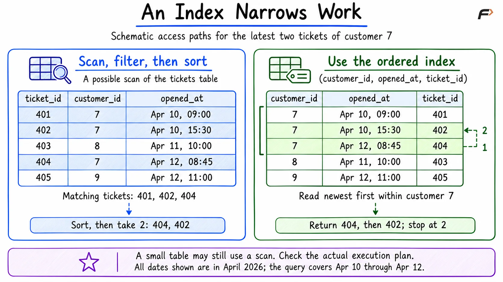
An Index Narrows Work
Run the same EXPLAIN ANALYZE again after creating the index. The optimizer may still choose a scan for this five-row table. Use representative data before drawing conclusions about performance.
Indexes also consume storage and add maintenance work to inserts, updates, and deletes. Choose them for useful query patterns rather than adding one to every column.
Keep Date Conditions Searchable
A condition is sargable when it can guide an index search. With an ordinary index on opened_at, applying DATE(opened_at) or casting the column to a date generally prevents that expression from directly defining a timestamp range in the index.
To count customer 7’s tickets opened on April 10, compare the stored timestamp with the day’s boundaries:
SELECT COUNT(*) AS tickets_openedFROM ticketsWHERE customer_id = 7 AND opened_at >= '2026-04-10 00:00:00' AND opened_at < '2026-04-11 00:00:00';Output: tickets_opened = 2, for tickets 401 and 402.
This half-open range includes the start of April 10 and excludes the start of April 11. It also includes any fractional-second timestamps before that upper boundary.
A function on opened_at does not mean every part of every index becomes unusable: the customer_id prefix may still help. A matching expression index is another possibility. The range form is a straightforward choice for this example.
Debug What the Result Rows Mean
A Join Can Change What You Are Counting
Each ticket can have several comments. The ticket_comments table contains:
comment_id | ticket_id |
|---|---|
1 | 401 |
2 | 401 |
3 | 401 |
4 | 402 |
5 | 403 |
Before adding a count, inspect the matching rows. The aliases t and c keep references to tickets and ticket_comments concise.
SELECT t.ticket_id, c.comment_idFROM tickets AS tJOIN ticket_comments AS c ON c.ticket_id = t.ticket_idWHERE t.customer_id = 7ORDER BY t.ticket_id, c.comment_id;Output
ticket_id | comment_id |
|---|---|
401 | 1 |
401 | 2 |
401 | 3 |
402 | 4 |
The join produces one row per matching comment. Ticket 401 appears three times, while ticket 404 disappears because it has no comments.
The counts answer different questions:
Calculation | Result | Meaning |
|---|---|---|
COUNT(*) over this join | 4 | Matching comment rows |
COUNT(DISTINCT t.ticket_id) over this join | 2 | Tickets with at least one comment |
COUNT(*) directly from customer 7’s tickets | 3 | All of that customer’s tickets |
The diagram makes both effects visible: one ticket can produce several joined rows, and an unmatched ticket can produce none.
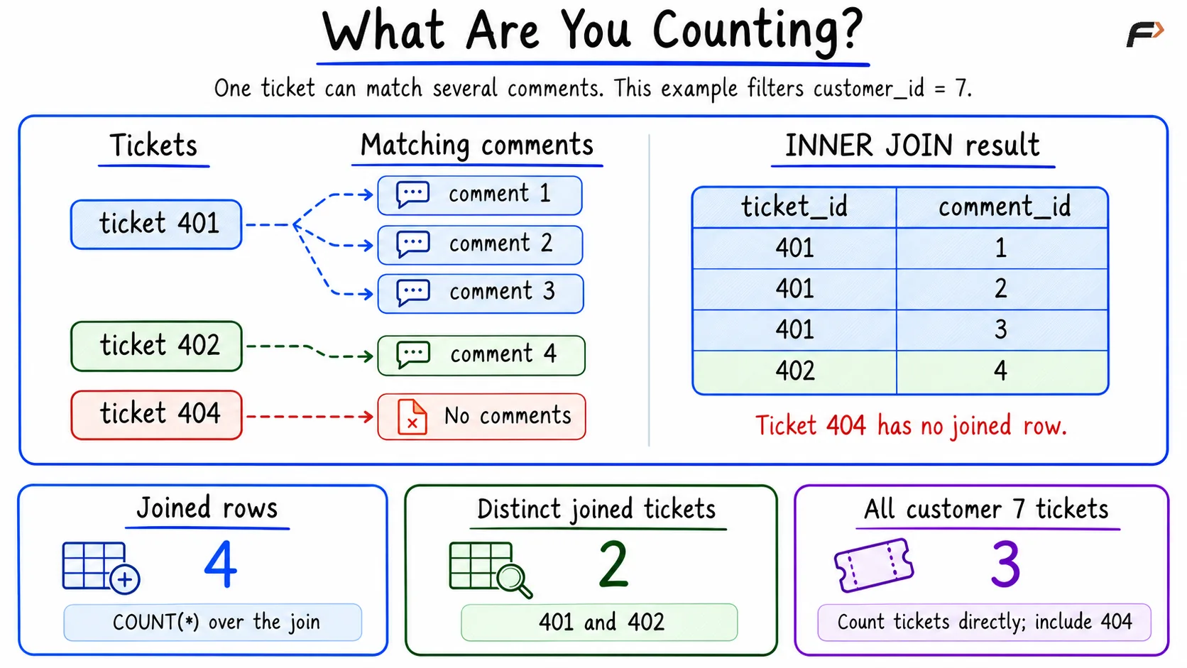
What Are We Counting
If the requirement is to count all tickets, query tickets directly:
SELECT COUNT(*) AS ticket_countFROM ticketsWHERE customer_id = 7;Output: ticket_count = 3.
Removing an unnecessary join fixes the meaning and removes work. Adding DISTINCT to an inner join would not restore ticket 404.
NULL Can Explain an Unexpected Empty Result
Suppose blocked_customers contains customer IDs 8 and NULL. We want tickets whose customer has no matching blocked record.
Using NOT IN against these two values produces FALSE for customer 8 and UNKNOWN for customers 7 and 9. Because WHERE keeps only TRUE, no ticket survives that filter. This follows SQL’s NULL rules.
Use NOT EXISTS to express the absence of a matching customer ID:
SELECT t.ticket_idFROM tickets AS tWHERE NOT EXISTS ( SELECT 1 FROM blocked_customers AS b WHERE b.customer_id = t.customer_id)ORDER BY t.ticket_id;Output: 401, 402, 404, 405, in that order. Ticket 403 is excluded because its customer ID is 8. The NULL blacklist entry does not create an equality match.
The comparison below shows why the two conditions give different results for this data.
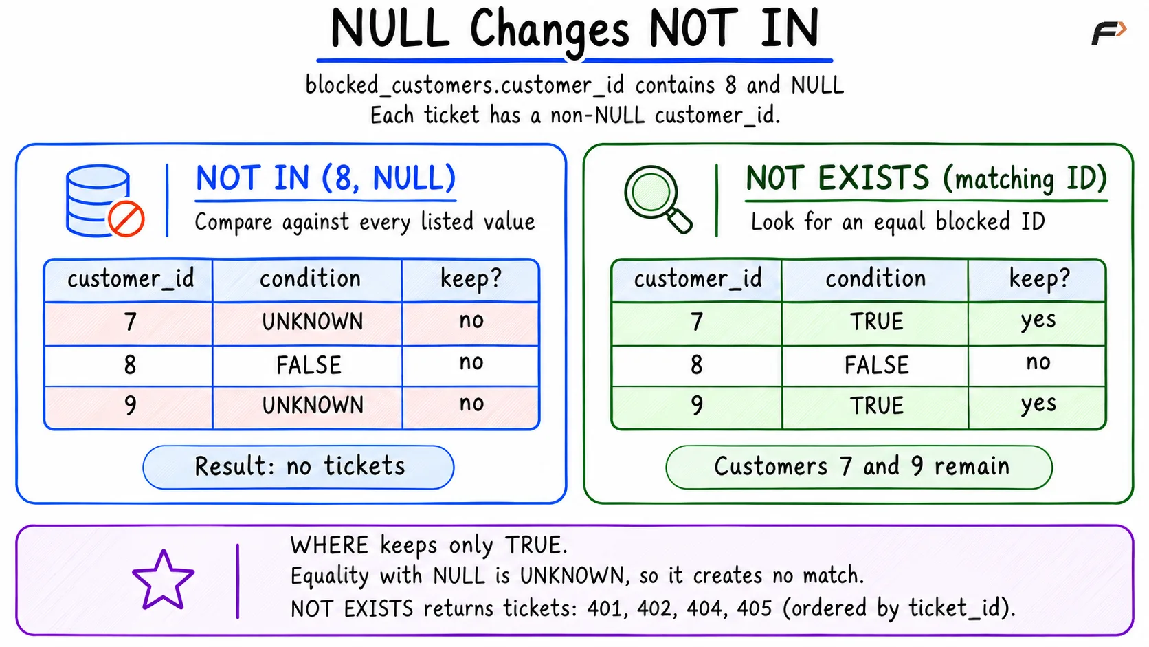
NULL Changes NOT IN
Filtering NULL values out of the NOT IN subquery is also valid here because tickets.customer_id is NOT NULL. If outer IDs can be NULL, decide how those rows should be handled before choosing a rewrite.
Use a Repeatable Debugging Routine
Confirm the expected result: Check identifiers, date boundaries, NULL values, and what one result row represents. Inspect joined rows before aggregating.
Record a baseline: Save the query, parameters, execution plan, and measured time using representative data.
Make one focused change: Rewrite a filter, remove an unnecessary join, or add an index that matches the query.
Compare again: Check that results remain correct and repeat measurements under similar conditions. Cache state and concurrent activity can affect timings.
Investigate waiting when necessary: If the application remains slow despite a quick query execution, check lock waits, connection delays, and how much data the application transfers.
If the query runs inside a stored procedure, inspect its SQL using the same parameter values. Procedures package reusable database logic and can reduce application-to-database calls, but they do not automatically improve an inefficient query. In MySQL, BEGIN ... END groups statements; it does not itself make them one atomic transaction.
Summary
SQL performance and debugging begin with knowing the expected result. Execution plans reveal how the database approaches a query, while EXPLAIN ANALYZE measures an actual execution. Useful indexes and searchable filters can reduce work, but join multiplicity and NULL handling must also preserve the intended answer. Make focused changes, verify the results, and compare measurements on representative data.
Be the first to add a comment.