Introduction
Database reports often need information about categories rather than individual records. An academic report might require the number of students in each department or the average marks for each department and semester.
GROUP BY organizes related rows into groups. Aggregate functions can then calculate a separate count, total, average, minimum, or maximum for each group.
An Example Relation
Consider an existing table named StudentResult. Each row stores a student’s department, semester, and marks in a common assessment.
StudentResult : initial data
StudentID | Name | Department | Semester | Marks |
|---|---|---|---|---|
101 | Asha | Computer Science | 2 | 80.00 |
102 | Ravi | Electronics | 4 | 60.00 |
103 | Meera | Computer Science | 2 | 90.00 |
104 | Arjun | Electronics | 2 | 70.00 |
105 | Neha | Computer Science | 4 | NULL |
106 | Kabir | Computer Science | 4 | 75.00 |
StudentID uniquely identifies each student. Marks stores decimal values, and Neha’s NULL means that her marks have not been recorded.
The table contains four Computer Science students and two Electronics students. These department values provide a natural basis for grouping.
Understanding GROUP BY Through Buckets
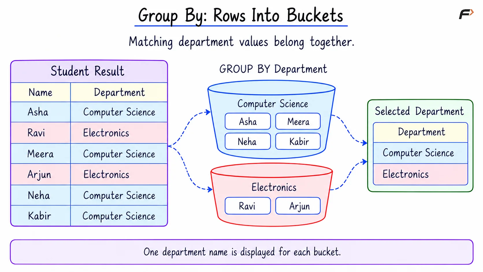
A simple way to visualize GROUP BY is to imagine labelled buckets. Each record goes into the bucket matching its grouping value.
With GROUP BY Department, the records form two buckets:
Computer Science: Asha, Meera, Neha, and Kabir.
Electronics: Ravi and Arjun.
The department name is the bucket’s label. A count describes how many records the bucket contains, while an average summarizes the recorded marks inside it.
A grouped summary therefore displays one result row for each bucket that remains after any group filtering.
Basic GROUP BY with SELECT and FROM
GROUP BY can be used without an aggregate function. Selecting the grouping column displays one value for each group.
In the StudentResult table, department names appear in several records. The requirement is to display each represented department once.
Consider the following queries to group the student records by department and display the department names.
SELECT DepartmentFROM StudentResultGROUP BY Department;Expected result
Department |
|---|
Computer Science |
Electronics |
Each clause has a specific role:
SELECT Department: Displays the department column.FROM StudentResult: Identifies the source table.GROUP BY Department: Places records with matching department values into the same group.
The four Computer Science records belong to one bucket, while the two Electronics records belong to another. Because the query displays only the grouping column, each department name appears once.
GROUP BY : ROWS INTO BUCKETS
Using Aggregate Functions with GROUP BY
An aggregate function calculates one result from the rows in a group. GROUP BY determines which rows contribute to each calculation.
Expression | Calculation within each group |
|---|---|
| Counts all rows |
| Counts non- |
| Adds the recorded marks |
| Calculates the average recorded marks |
| Finds the lowest recorded marks |
| Finds the highest recorded marks |
Consider the following queries to calculate each department’s student count, recorded-result count, and average marks.
SELECT Department AS department, COUNT(*) AS student_count, COUNT(Marks) AS graded_count, ROUND(AVG(Marks), 2) AS average_marksFROM StudentResultGROUP BY DepartmentORDER BY Department;Expected result
department | student_count | graded_count | average_marks |
|---|---|---|---|
Computer Science | 4 | 3 | 81.67 |
Electronics | 2 | 2 | 65.00 |
In COUNT(*), the * means that rows are counted regardless of their column values. AS assigns readable output names, and ROUND(AVG(Marks), 2) rounds the average to two decimal places.
The Computer Science bucket contains four students but only three recorded marks: 80, 90, and 75. Their total is 245, so the average is approximately 81.67.
Without GROUP BY, an aggregate query can summarize all qualifying rows together instead of producing a separate summary for each department.
Grouping by Multiple Columns
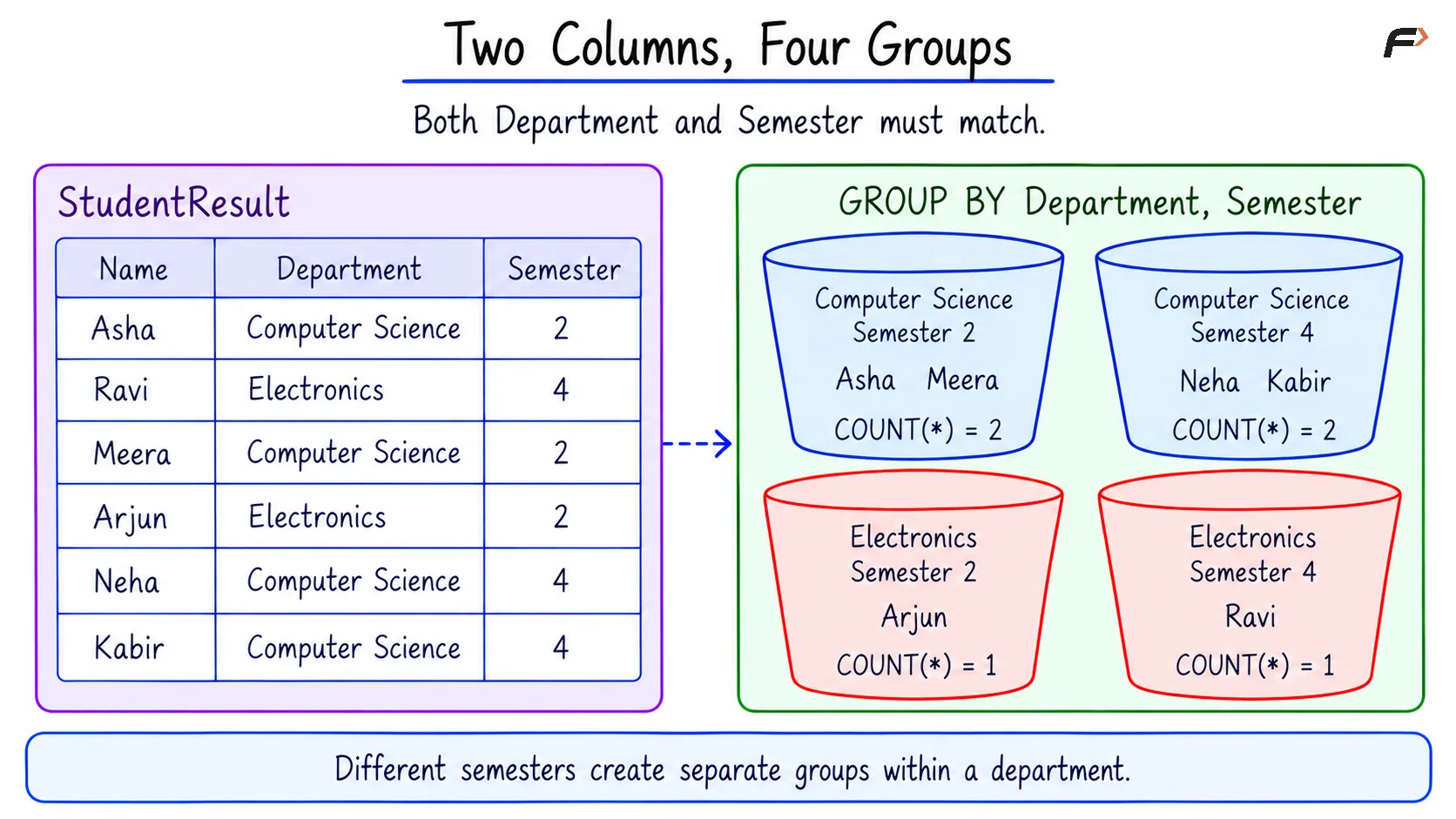
Grouping by multiple columns creates a separate group for each distinct combination of their values.
The bucket label now contains more than one value. With GROUP BY Department, Semester, the labels include Computer Science, semester 2 and Computer Science, semester 4. These are separate groups even though their department names match.
Consider the following queries to count students in each department-semester combination.
SELECT Department AS department, Semester AS semester, COUNT(*) AS student_countFROM StudentResultGROUP BY Department, SemesterORDER BY Department, Semester;Expected result
department | semester | student_count |
|---|---|---|
Computer Science | 2 | 2 |
Computer Science | 4 | 2 |
Electronics | 2 | 1 |
Electronics | 4 | 1 |
Asha and Meera belong to the Computer Science, semester 2 group. Neha and Kabir belong to the Computer Science, semester 4 group.
Grouping only by department produced two groups. Adding semester produces four groups, giving the report a finer level of detail.
TWO COLUMNS , FOUR GROUPS
Choosing Columns for a Grouped Result
The output should contain values that clearly describe each group. The usual choices are the grouping columns and aggregate results.
For straightforward, portable queries, include each selected non-aggregated column in GROUP BY. In the previous example, both Department and Semester appear in the output and in the grouping clause.
An individual Name would not describe an entire department containing several students. Adding Name to GROUP BY changes the report to department-and-name groups; it does not preserve the department-wide summary.
Similarly, grouping by the unique StudentID would create one group per student, which would not provide a department-level overview.
How GROUP BY Handles NULL
A missing value can occur either in a grouping column or in the column being summarized.
Missing grouping value: If
DepartmentcontainsNULLvalues,GROUP BY Departmentplaces those records together in oneNULLdepartment group. With multiple grouping columns, the other grouping values must also match.Missing aggregate input: A row with
NULLmarks still belongs to its department’s group.COUNT(*)includes the row, butCOUNT(Marks),SUM(Marks),AVG(Marks),MIN(Marks), andMAX(Marks)ignore its missing marks.
If a group contains no recorded marks, COUNT(Marks) returns 0, while the other four aggregate functions return NULL. An unknown mark should not automatically be treated as zero because that changes the calculation.
Relation of WHERE and HAVING with GROUP BY
WHERE and HAVING control different parts of a grouped query.
Clause | Role in a grouped query | Example |
|---|---|---|
| Selects individual rows that can enter the groups |
|
| Selects groups after their summaries are calculated |
|
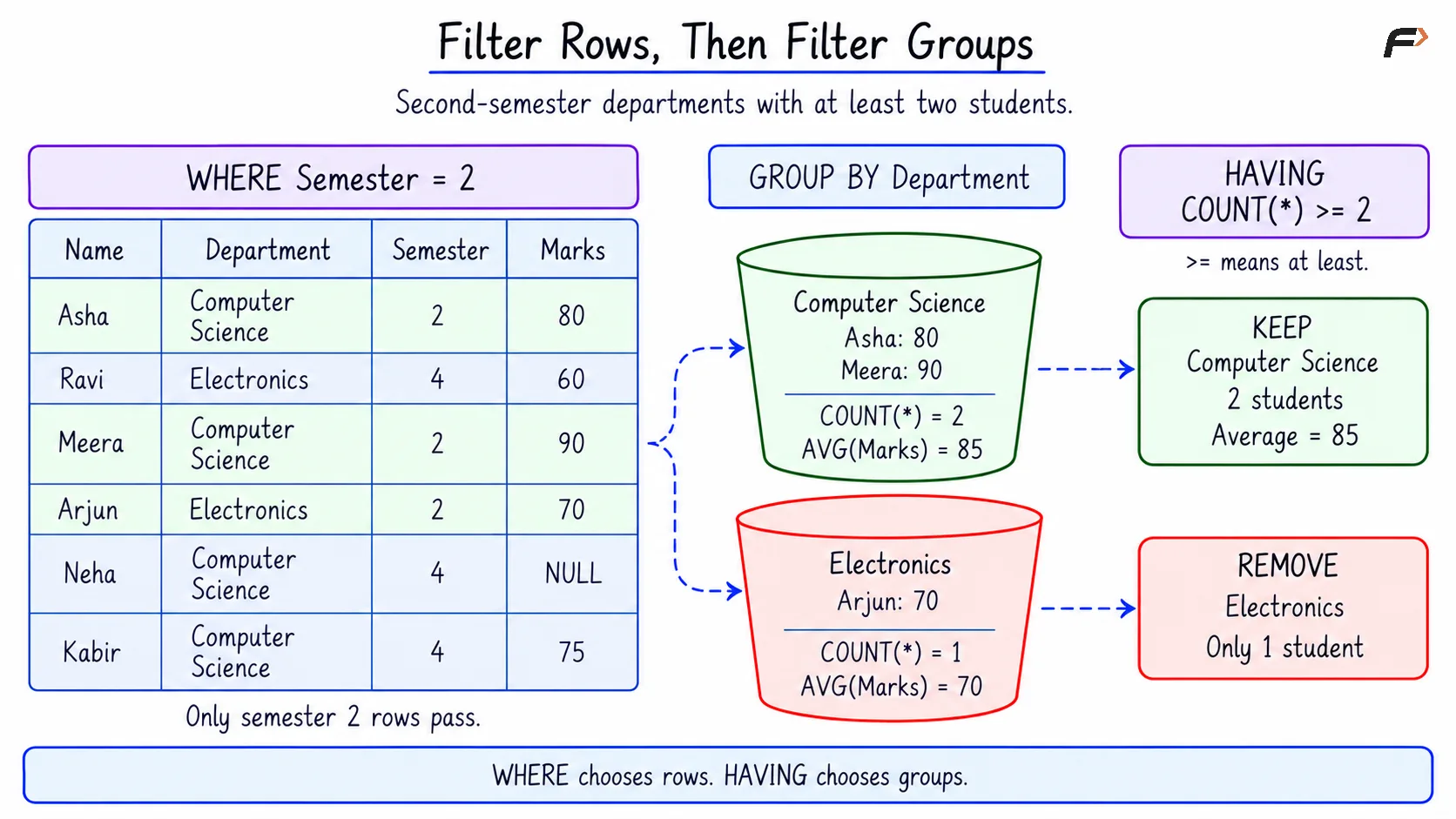
Using the bucket analogy, WHERE decides which records are allowed into the buckets. HAVING decides which completed buckets should appear in the report.
For example, WHERE Semester = 2 keeps only second-semester students. After grouping those students by department, HAVING COUNT(*) >= 2 keeps departments containing at least two qualifying students.
Here, = tests equality and >= means “greater than or equal to.” A condition on the current group’s count or average belongs in HAVING, because it depends on the group’s calculated result.
GROUP BY, DISTINCT, and ORDER BY
These clauses serve different purposes:
Clause | Main purpose | Typical use |
|---|---|---|
| Forms groups for summaries | Count students in each department |
| Removes duplicate output rows | Display each department name once |
| Sorts the output rows | Arrange departments alphabetically |
Selecting distinct department names can produce the same department values as grouping by department and displaying that column alone. GROUP BY is especially useful when each category also needs its own calculated summary.
Grouping does not automatically sort the results. ORDER BY specifies the display order; ASC means ascending order, and DESC means descending order.
A Compact Example
The relevant data is repeated below for reference.
StudentID | Name | Department | Semester | Marks |
|---|---|---|---|---|
101 | Asha | Computer Science | 2 | 80.00 |
102 | Ravi | Electronics | 4 | 60.00 |
103 | Meera | Computer Science | 2 | 90.00 |
104 | Arjun | Electronics | 2 | 70.00 |
105 | Neha | Computer Science | 4 | NULL |
106 | Kabir | Computer Science | 4 | 75.00 |
The requirement is to find departments containing at least two second-semester students, display their student count and average recorded marks, and sort the report by average marks from highest to lowest.
Consider the following queries to create the departmental summary for second-semester students.
SELECT Department AS department, COUNT(*) AS student_count, ROUND(AVG(Marks), 2) AS average_marksFROM StudentResultWHERE Semester = 2GROUP BY DepartmentHAVING COUNT(*) >= 2ORDER BY average_marks DESC, department ASC;Expected result
department | student_count | average_marks |
|---|---|---|
Computer Science | 2 | 85.00 |
WHERE keeps Asha, Meera, and Arjun because their semester is 2. GROUP BY places Asha and Meera in the Computer Science bucket and Arjun in the Electronics bucket.
Computer Science has two qualifying students, with an average of 85. Electronics has only one qualifying student, so HAVING COUNT(*) >= 2 excludes it.
ORDER BY sorts the surviving summaries by average marks. Department names provide an ascending tie-breaker when averages match. Only one department qualifies in this example.
FILTER ROWS THEN FILTER GROUPS
Summary
GROUP BY organizes rows into groups based on one or more column values. Thinking of these groups as labelled buckets makes it easier to understand how aggregate functions calculate a separate result for each category.
The grouping columns determine the report’s level of detail. WHERE controls which rows contribute, HAVING controls which groups remain, and ORDER BY arranges the final summaries. Correct handling of NULL and appropriate output columns keep the results meaningful.
Be the first to add a comment.