Introduction
A college database can store information about thousands of students and their departments. Retrieving useful information requires operations such as finding students from a particular department, displaying selected attributes, or combining student records with department details. Relational algebra provides a precise way to express these requests.
Fundamental relational algebra consists of a small set of operations that take relations as input and produce relations as output. These operations explain the logical structure of database queries and provide a foundation for understanding SQL, joins, and query optimization.
What Is Relational Algebra in DBMS?
Relational algebra is a formal, procedural query language that defines operations on relations. An expression specifies which logical operations to apply and how their results feed into other operations.
For example, a query can first identify students in their second semester and then retain only their names. This describes a logical procedure. It does not prescribe physical details such as which index to use or which join algorithm the DBMS should execute.
Three ideas are central to classical relational algebra:
Closure: Every operation produces another relation, so its output can become the input to another operation.
Set semantics: Relations contain distinct tuples. Duplicate tuples are not retained, and row order has no significance.
Result construction: Query operations produce a result relation without changing the stored input relations.
An operator that takes one relation is unary, while an operator that takes two relations is binary. This classification depends on the number of input relations, rather than the number of attributes or conditions mentioned.
Example Relations
Consider the following relations from a college database. These records will be used throughout the examples so that the effect of each operator remains easy to follow.
Student :
StudentID | Name | DeptID | Semester |
|---|---|---|---|
101 | Asha | 10 | 2 |
102 | Ravi | 20 | 4 |
103 | Meera | 10 | 2 |
Department :
DeptID | DeptName |
|---|---|
10 | Computer Science |
20 | Electronics |
In these relations, a tuple is a row and an attribute is a column. The DeptID attribute connects each student to the corresponding department.
The expressions below place operator conditions and attribute lists inside square brackets for readability. For example, σ[DeptID = 10](Student) means applying selection to Student with the condition DeptID = 10.
The Six Fundamental Relational Algebra Operations
A commonly used foundation for relational algebra contains six operators. More complex operations can be expressed by combining these building blocks:
Unary operators: Selection (
σ), projection (π), and rename (ρ).Binary operators: Union (
∪), set difference (−), and Cartesian product (×).
Each operator has its own purpose and requirements. Choosing the correct operator depends on whether the query needs to filter rows, retain attributes, combine compatible records, or form combinations across relations.
Selection: Filtering Rows
The selection operator, represented by sigma (σ), retains tuples that satisfy a condition. Its general form is σ[condition](R), where R is the input relation.
To retrieve students belonging to department 10, use:
σ[DeptID = 10](Student)The result is:
StudentID | Name | DeptID | Semester |
|---|---|---|---|
101 | Asha | 10 | 2 |
103 | Meera | 10 | 2 |
Selection preserves all attributes of the input relation. It may return fewer rows, all rows, or no rows, depending on the condition. An empty result still has the same schema as the input.
Conditions can use comparisons such as =, ≠, <, >, ≤, and ≥. They can also combine predicates using AND (∧), OR (∨), and NOT (¬). For example, σ[DeptID = 10 ∧ Semester = 2](Student) requires both conditions to hold.
Projection: Choosing Columns
The projection operator, represented by pi (π), retains specified attributes. Its general form is π[attribute list](R). Attributes that are not listed are excluded from the result.
To retrieve the department IDs appearing in the student relation, use:
π[DeptID](Student)The result is:
DeptID |
|---|
10 |
20 |
Although department 10 appears in two student records, it appears only once in this result. Projection eliminates duplicate output tuples because classical relational algebra uses set semantics.
When several attributes are projected, duplicate elimination considers their complete combination. For example, π[Name, DeptID](Student) retains distinct name-department pairs; it does not independently remove repeated values from each column.
The difference between selection and projection is:
Aspect | Selection | Projection |
|---|---|---|
Main purpose | Retains rows satisfying a condition. | Retains specified columns. |
Output attributes | Same as the input relation. | Only the listed attributes. |
Effect on tuples | Filters existing tuples. | Can collapse tuples that become identical after columns are removed. |
Example |
|
|
Both operations can reduce the number of tuples, but only projection changes which attributes appear in the result.
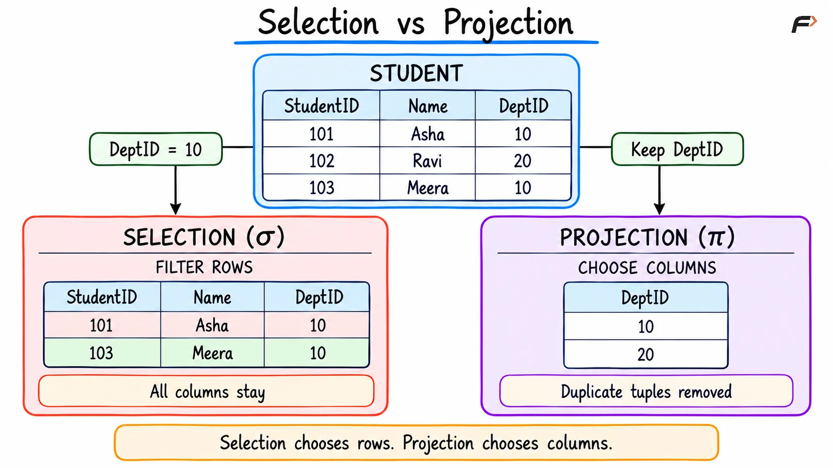
SELECTION VS PROJECTION
Union: Combining Compatible Relations
The union operator returns every tuple that appears in either input relation, including tuples that appear in both. Each distinct tuple occurs only once in the result.
Union requires union-compatible relations:
Same degree: Both relations must contain the same number of attributes.
Matching domains: Corresponding attributes must have matching domains.
Aligned attributes: When using named attributes, rename them where necessary so the schemas align.
Consider two relations with the same schema, StudentID:
DBMSClub:
{(101), (102)}CodingClub:
{(102), (103)}
Their union is DBMSClub ∪ CodingClub = {(101), (102), (103)}. Student 102 appears once even though the student belongs to both clubs.
Union is commutative: R ∪ S = S ∪ R. If the input schemas are incompatible, the operation is undefined; it does not produce a NULL result.
Set Difference: Finding Tuples Present Only in the First Relation
The set difference operator, written as R − S, returns tuples that belong to R but do not belong to S. Like union, it requires union-compatible inputs.
Using the club relations:
DBMSClub − CodingClub = {(101)}: Student 101 belongs to the DBMS club but not the coding club.CodingClub − DBMSClub = {(103)}: Student 103 belongs to the coding club but not the DBMS club.
Set difference is not commutative. Reversing the operands changes which relation supplies the candidate tuples and which relation excludes them.
Tuple comparison uses all attributes in the input schema. To compare only student IDs from larger relations, first project the StudentID attribute from both sides, then apply set difference.
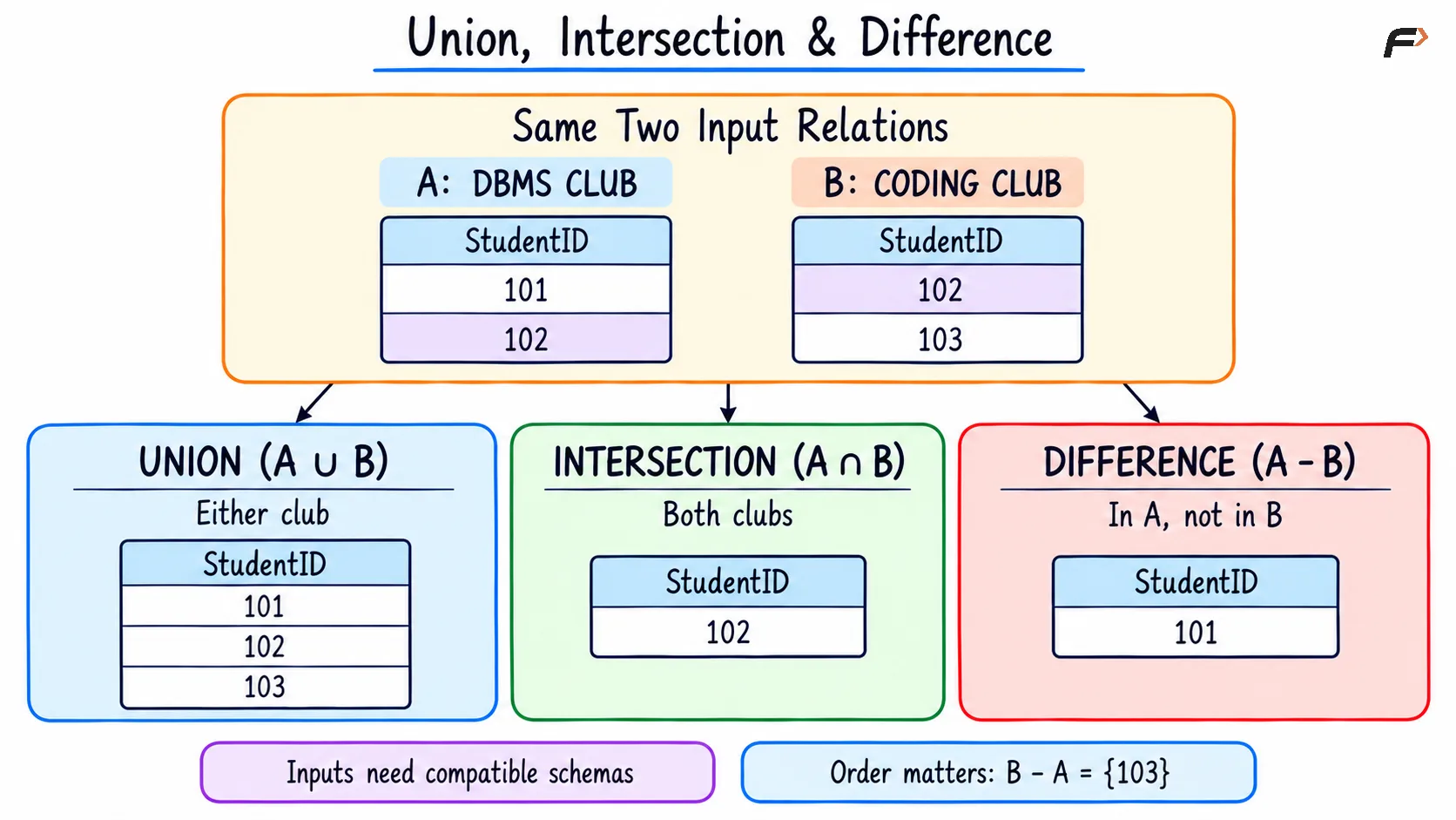
Union, Intersection and Difference
Cartesian Product: Forming Every Possible Pair
The Cartesian product, represented by ×, combines every tuple of one relation with every tuple of another. It does not apply a matching condition.
For the sample data, Student × Department pairs each of the three students with both departments. Asha therefore appears once alongside Computer Science and once alongside Electronics, even though her recorded department ID is 10.
For relations R and S:
Result cardinality: If
Rhasmtuples andShasntuples, the product containsm × ntuples.Result degree: The number of attributes is the sum of the degrees of the two inputs.
Here, the product contains 3 × 2 = 6 tuples and 4 + 2 = 6 attributes. If either input relation is empty, the product is also empty.
Unlike union, Cartesian product does not require compatible schemas. However, attributes must remain distinguishable. Because both sample relations contain DeptID, use qualified names such as Student.DeptID and Department.DeptID, or rename conflicting attributes.
A matching condition applied after the product can retain only related student-department pairs. This provides the basis for a theta join.
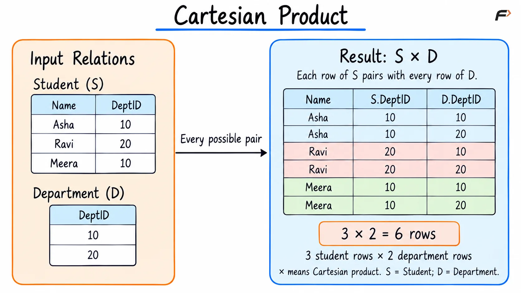
CARTESIAN PRODUCT
Rename: Giving Relations and Attributes Clear Names
The rename operator, represented by rho (ρ), changes the name of a result relation, its attributes, or both. It preserves the tuple values, cardinality, and degree.
For example, ρ[S](Student) gives the student relation the name S within an expression. To rename both a relation and one of its attributes, use:
ρ[D(DepartmentID, DeptName)](Department)The resulting relation is named D. Its attributes are DepartmentID and DeptName, corresponding to the original DeptID and DeptName attributes.
Rename is useful when combining relations with overlapping attribute names or when using the same relation more than once, as in a self-join. It changes the names used in the expression rather than permanently altering a stored table.
Rename remains a unary operation because it takes one input relation, even when several new names are specified.
Combining Relational Algebra Operations
The closure property allows operators to be nested. Consider the request: retrieve the names and department names of students in semester 2.
One expression is:
π[Student.Name, Department.DeptName]( σ[Student.DeptID = Department.DeptID ∧ Student.Semester = 2]( Student × Department ))Read the expression from the innermost operation outward. The product forms six student-department pairs. Selection retains the two pairs with matching department IDs and semester 2. Projection then keeps the requested attributes.
The result is:
Name | DeptName |
|---|---|
Asha | Computer Science |
Meera | Computer Science |
Different expressions can produce the same result. Filtering Student to semester 2 before forming the product reduces this example’s intermediate combinations from six to four. Such equivalences help a query optimizer consider alternative logical plans.
Two successive selections can also be combined: σ[p](σ[q](R)) = σ[p ∧ q](R). Their order can be exchanged because both conditions must ultimately hold.
Projection needs more care. If Semester is removed before evaluating Semester = 2, the later selection cannot access that attribute. Any rewrite must preserve the attributes needed by subsequent operations.
Derived Operations: Intersection, Join, and Division
The six fundamental operators can express additional operations. These derived operators make common query patterns shorter and easier to read.
Intersection (
∩): Returns tuples present in both compatible relations. It can be expressed asR ∩ S = R − (R − S). For the club example, the intersection contains only student 102.Theta join (
⋈): Combines tuples that satisfy a specified condition. Its definition isR ⋈[condition] S = σ[condition](R × S). An equijoin is a theta join whose matching conditions use equality.Division (
÷): Expresses “for every” requirements. GivenEnrollment(StudentID, CourseID)andRequired(CourseID),Enrollment ÷ Requiredreturns student IDs associated with every course listed inRequired.
A natural join matches values on all common attribute names and retains one copy of each shared attribute. It can be constructed using Cartesian product, selection, projection, and appropriate renaming.
The Cartesian product includes every possible pair, while a join retains pairs satisfying its matching rule. The algebraic definition does not require a DBMS to physically materialize the entire product; an implementation can use a suitable join algorithm.
Operations such as grouping, aggregation, and outer joins belong to extended relational algebra. They add capabilities beyond the six fundamental operators discussed here.
A Compact Example
Consider the request: retrieve the names and department names of students in semester 2. Assuming the Student and Department tables contain the sample records, the following queries produce the same result as the relational algebra expression discussed earlier.
SELECT DISTINCT s.Name, d.DeptNameFROM Student AS sJOIN Department AS d ON s.DeptID = d.DeptIDWHERE s.Semester = 2;The JOIN condition matches each student to a department, WHERE filters students by semester, and the select list retains the requested columns. DISTINCT removes duplicate output rows, matching the set semantics of classical projection.
The main differences to remember are:
Aspect | Classical relational algebra | SQL |
|---|---|---|
Query description | Specifies a composition of logical operators. | Declaratively describes the desired result. |
Duplicate tuples | Relations and results contain no duplicate tuples. | Ordinary |
Row order | Relations have no inherent row order. | A particular output order requires |
Missing information | The basic model assumes domain values without SQL | Supports |
Despite its name, relational algebra’s selection corresponds to SQL’s WHERE filtering. SQL’s select list performs the column-selection role of projection, with DISTINCT providing duplicate elimination when needed.
Summary
Fundamental relational algebra uses selection, projection, union, set difference, Cartesian product, and rename to construct query results. These operators work on relations and return relations, allowing simple operations to be combined into larger expressions.
Correct expressions depend on set semantics, compatible schemas, clear attribute names, and a valid order of operations. Understanding these foundations makes it easier to distinguish filtering from projection, products from joins, and logical query expressions from their SQL implementations.
Be the first to add a comment.