Introduction
Routing in a large network cannot depend only on partial information. If a router knows only what its neighbors tell it, route calculation becomes slower, less reliable, and harder to scale. That is why Link State Routing became so important in modern networks.
In Link State Routing, each router learns the complete network map and then calculates the best path on its own. This is very different from older distance vector methods, where routers depend heavily on neighbor updates. OSPF, or Open Shortest Path First, is the most widely used protocol based on this idea.
What Is Link State Routing?
Link State Routing is a dynamic routing approach in which every router builds a view of the full network topology. After learning how routers are connected and what each link costs, the router computes the shortest path to every destination.
The basic idea is simple:
Every router describes its own local links.
That information is shared across the network.
Routers in the same OSPF area build the same link-state database for that area.
Each router calculates the best routes independently.
So instead of asking, "What route do you know?", a router effectively says, "Tell me the network map, and I will calculate the best path myself."
Distance Vector vs Link State
Both approaches are used to find routes, but they work very differently.
Feature | Distance Vector Routing | Link State Routing |
|---|---|---|
Network knowledge | Partial, based on neighbors | Full topology view |
Route learning | Learns from neighbor advertisements | Learns from network-wide link information |
Path calculation | Indirect | Direct shortest-path calculation |
Convergence | Usually slower | Usually faster |
Scalability | Better for small networks | Better for large networks |
Example | RIP | OSPF |
Link State Routing is preferred in larger and more complex networks because it gives routers better visibility and better control over path selection.
Why Link State Routing Is Needed
Distance vector protocols are simple, but they start showing limitations as the network grows.
Some common problems are:
Slow convergence: Routers may take longer to agree on changes after a failure.
Routing loops: Outdated information can circulate and cause incorrect forwarding.
Limited visibility: Routers do not know the full network structure.
Poor scalability: Some distance vector protocols have practical limits in bigger networks.
Link State Routing solves these problems by giving routers a complete picture of the network.
How Link State Routing Works
The operation of Link State Routing can be understood in a clear sequence.
1. Neighbor Discovery
Each router first discovers the routers directly connected to it. These are its immediate neighbors.
For example, a router may find that it is connected to three nearby routers through different interfaces.
2. Link Cost Calculation
The router then checks each connection and assigns a cost to it. This cost is often based on bandwidth, though other design choices may also influence it.
At this point, the router knows:
Which links are active
Which neighbors are reachable
What cost is associated with each link
3. LSA Creation
The router creates a Link State Advertisement, or LSA. This message describes the router's local links and their costs.
A simple example might look like this:
R1 => R2 : Cost 2
R1 => R3 : Cost 5
R1 => R4 : Cost 1
Every router creates its own LSA in a similar way.
4. Flooding the LSA
The LSA is not sent to only one router. It is flooded through the network so that all routers receive the same link-state information.
Flooding ensures that routers in the same area learn the same link-state information for that area.
5. Topology Database Formation
After receiving LSAs from all routers, each router builds a topology database. This database represents the network map.
It contains:
Routers
Links between routers
Costs of those links
Because all routers receive the same advertisements, they build a consistent view of the network.
6. Shortest Path Calculation
Now the router has enough information to calculate the shortest path to every destination. This is usually done using Dijkstra's Algorithm.
The router computes the best route from itself to all other routers based on total path cost.
7. Routing Table Update
Finally, the best paths are placed into the routing table. The router then uses this table to forward packets efficiently.
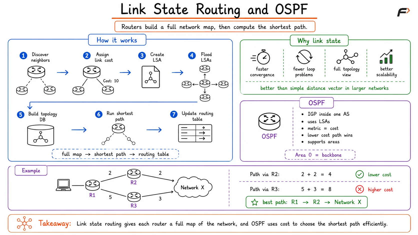
Link State Routing and OSPF
Dijkstra's Algorithm in Simple Terms
Dijkstra's Algorithm is the shortest-path method commonly associated with link state routing.
You can think of it like finding the cheapest route on a full road map. If you already know all cities, roads, and road lengths, you can calculate the shortest route from your city to every other city. Link State Routing does the same thing in a network.
That is why Link State Routing works in this order:
Full network map => Shortest path calculation => Routing table creation
What Is OSPF?
OSPF stands for Open Shortest Path First. It is a link state Interior Gateway Protocol used inside a single autonomous system.
OSPF is one of the most widely used routing protocols in enterprise networks because it converges quickly, handles large topologies well, and supports structured network design.
OSPF uses LSAs to exchange topology information, builds a link-state database, and computes shortest paths using cost as its metric.
Key Features of OSPF
OSPF includes several important features that make it suitable for modern networks:
It is an IGP: Used within one autonomous system.
It is link state based: Routers build a complete topology view.
It uses LSAs: Routers advertise local link information.
It uses cost as a metric: Lower total cost paths are preferred.
It supports hierarchical design: Networks can be divided into areas.
It converges quickly: Topology changes are handled efficiently.
It scales well: Better suited for large networks than simple distance vector protocols.
OSPF Cost
OSPF selects routes based on cost, not hop count. In general, a lower-cost path is preferred over a higher-cost path.
This is an important improvement over protocols that rely only on the number of hops. A path with fewer hops is not always the best path if link quality or bandwidth is poor.
OSPF Areas
One of the major strengths of OSPF is area-based design. Instead of keeping the entire network as one flat structure, OSPF can divide it into areas.
This helps by:
Reducing routing overhead
Improving scalability
Making large networks easier to manage
The backbone area, Area 0, plays a central role in connecting other areas in OSPF.
Advantages of Link State Routing and OSPF
Link State Routing and OSPF offer several practical benefits:
Faster convergence after network changes
Better scalability in large networks
More accurate route selection
Full topology awareness
Lower chance of classic routing loop problems
Support for structured and hierarchical design
These benefits make OSPF a strong choice for medium and large internal networks.
Disadvantages of Link State Routing
Even though link state routing is powerful, it also has some costs:
More memory is required to store the topology database
More CPU is needed for shortest-path calculations
Configuration and troubleshooting are more complex
LSA flooding adds protocol overhead
So while Link State Routing is efficient, it is not as lightweight as simpler routing methods.
Summary
Link State Routing is a routing method in which routers learn the complete network topology, exchange link information, and calculate the shortest paths on their own. This gives routers better visibility, faster convergence, and stronger scalability than distance vector routing.
OSPF is the most important example of a link state routing protocol. It uses LSAs, cost-based path selection, topology databases, and Dijkstra's Algorithm to build efficient routes inside an autonomous system. In modern enterprise networking, OSPF remains one of the most reliable and widely used routing protocols.
Be the first to add a comment.