Parent and Distance in a Binary Tree
A binary tree normally stores connections from a node to its children:
Left child
Right child
These connections make downward traversal straightforward. However, many problems also require movement from a node to its parent.
Examples include:
Finding all nodes at distance
Kfrom a targetCalculating the distance between two nodes
Simulating fire or infection spreading through a tree
Finding the nearest leaf
Moving from a node toward its ancestors
To solve such problems, the tree can be viewed as an undirected structure in which every node may have up to three neighbours:
Left child
Right child
Parent
Understanding parent relationships and distance allows ordinary tree traversal techniques to solve a much wider range of problems.
Parent of a Node
The parent of a node is the node directly connected above it.
Consider a binary tree with the following relationships:
Node
1is the root.Nodes
2and3are the children of1.Nodes
4and5are the children of2.Node
6is the right child of3.Nodes
7and8are the children of5.
The parent relationships are:
Node | Parent |
|---|---|
|
|
|
|
|
|
|
|
|
|
|
|
|
|
|
|
The root has no parent, so its parent is represented as NULL.
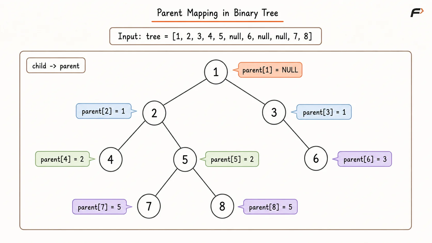
Parent Mapping in Binary Tree.png
Why Is a Parent Mapping Required?
A typical binary-tree node stores references only to its children. If traversal begins from the root, the recursive call stack remembers how to return to a parent.
However, consider starting traversal directly from target node 5.
Using only the node structure, we can move to:
Left child
7Right child
8
We cannot directly move upward to node 2 because node 5 does not store its parent.
A parent mapping stores the reverse relationship:
child → parent
After creating this mapping, node 5 has three possible neighbours:
7, 8, and 2
The tree can now be traversed outward from any selected node.
Constructing the Parent Mapping
A parent mapping can be constructed using either BFS or DFS from the root.
Whenever a node and one of its children are visited, store:
parent[child] = current node
The root is assigned no parent.
Algorithm
Return immediately if the tree is empty because there are no relationships to store.
Begin a BFS or DFS from the root and treat its parent as
NULL.Whenever a left child exists, record the current node as its parent.
Whenever a right child exists, record the current node as its parent.
Continue traversal until every node has been processed.
Use the completed mapping whenever upward movement is required.
Time Complexity: O(N) because every node is visited once.
Space Complexity: O(N) because one parent entry may be stored for every node.
Tree as an Undirected Graph
A binary tree is usually drawn with edges directed downward from parents to children. Structurally, however, every tree edge connects two nodes and can be travelled in either direction when both relationships are known.
After parent mapping, every node can be treated like a graph vertex.
For node 5:
Left neighbour:
7Right neighbour:
8Parent neighbour:
2
The original tree edge between 2 and 5 can now be followed as:
2 ↔ 5
This graph-like interpretation is the key idea behind distance-based traversal.
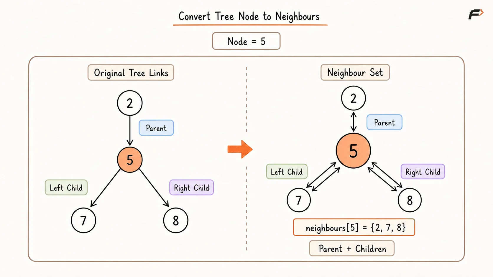
Convert Tree Node to Neighbours.png
Why Is a Visited Structure Necessary?
A normal downward tree traversal does not revisit a node because child references never lead back to the parent.
After parent links are introduced, movement becomes bidirectional.
For example:
5 → 2 → 5 → 2 → ...
Without a visited structure, traversal can repeatedly move between a node and its parent.
A visited set ensures that every node is processed only once.
A node should generally be marked as visited when it is added to the queue, not when it is removed. This prevents the same node from being added by multiple neighbours.
Understanding Distance
The distance between two nodes is the number of edges on the unique path connecting them.
In a tree, exactly one simple path exists between any two nodes.
Using the example tree:
Distance from
5to5is0.Distance from
5to2is1.Distance from
5to7is1.Distance from
5to1is2.Distance from
5to3is3.Distance from
5to6is4.
If a path contains P nodes, it contains:
P - 1 edges
Therefore, edge-based distance is one less than the number of nodes on the path.
Depth and Distance
Depth is a special form of distance.
The depth of a node is its distance from the root:
Depth of node X = Distance(root, X)
For example:
Depth of
1is0.Depth of
2is1.Depth of
5is2.Depth of
7is3.
Distance between two arbitrary nodes is not generally the difference between their depths. The path may first move upward to a common ancestor and then downward into another subtree.
Distance Layers from a Target Node
When BFS begins from a target node, each queue level represents one distance from that target.
Using target node 5:
Distance | Nodes |
|---|---|
|
|
|
|
|
|
|
|
|
|
These layers are formed because BFS processes nodes in increasing order of their distance from the starting node.
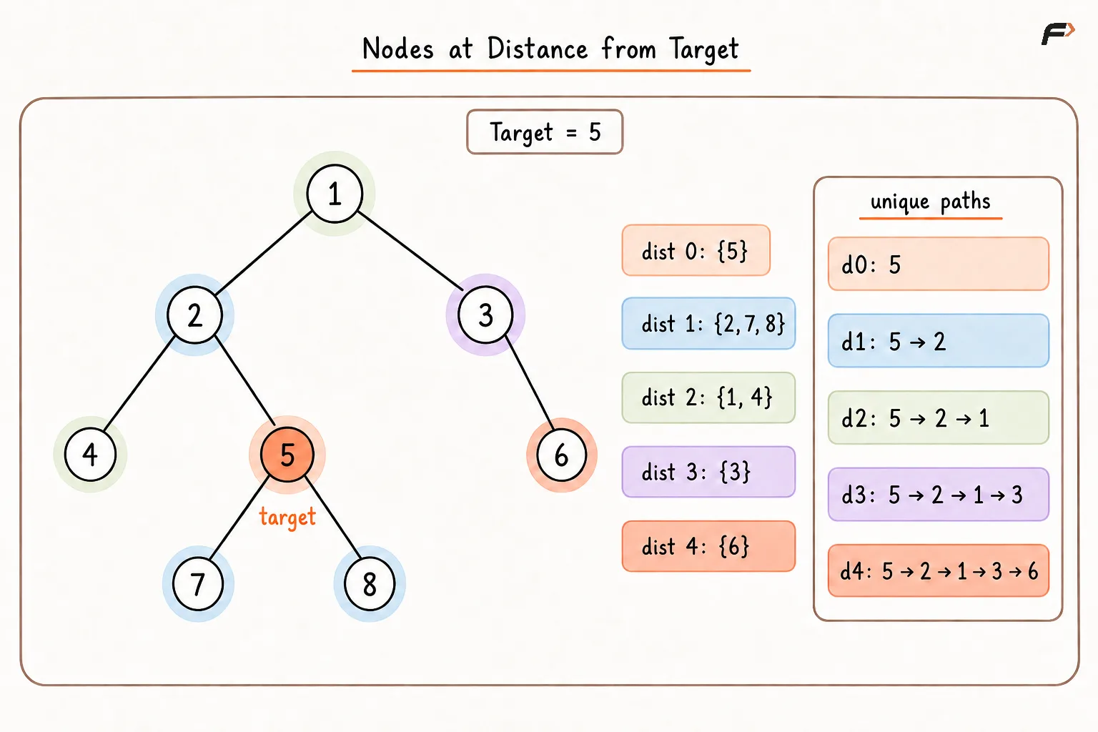
Nodes at Distance from Target .png
Finding Nodes at Distance K
Given a binary tree, a target node, and an integer K, find all nodes whose distance from the target is exactly K.
For the example tree:
Target = 5
K = 2
The nodes at distance 2 are:
1 and 4
Therefore:
Answer = [1, 4]
The order may depend on the order in which neighbours are added unless the problem requires a specific ordering.
Mental Model
The target node acts as the source of a BFS.
The target is at distance
0.Its unvisited neighbours are at distance
1.Their unvisited neighbours are at distance
2.The process continues until distance
Kis reached.
Once BFS has expanded exactly K levels, the nodes remaining in the current frontier are the required nodes.
Algorithm
Build a parent mapping for every node so traversal can move upward as well as downward.
Place the target node in a queue, mark it visited, and initialize the current distance to
0.Process one complete queue level at a time because each level represents one distance from the target.
For every node in the current level, add its unvisited left child, right child, and parent.
Increase the distance after the complete level has been processed.
Stop after reaching distance
K; the current queue contains exactly the required nodes.
Dry Run: Nodes at Distance 2 from Node 5
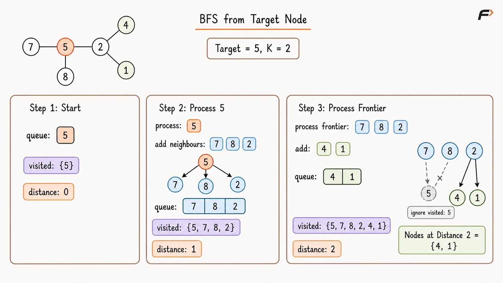
BFS from Target Node.png
Why Does the BFS Method Work?
Once parent links are available, the tree behaves like an unweighted graph.
BFS processes nodes in increasing order of the number of edges from the target:
The initial node has distance
0.Nodes discovered during the first expansion have distance
1.Nodes discovered during the second expansion have distance
2.
Because every tree edge has equal weight, the first time a node is discovered gives its shortest and only simple-path distance from the target.
Therefore, after exactly K level expansions, the queue contains all and only the nodes at distance K.
Complexity Analysis
Building the parent mapping takes:
O(N) time and O(N) space.
The BFS from the target may visit every node:
O(N) time and O(N) space.
Therefore, the complete complexity is:
Time Complexity: O(N)
Space Complexity: O(N)
The answer list is output space and is excluded from auxiliary space unless stated otherwise.
Important Edge Cases
K Equals 0
The target itself is the only node at distance 0.
Answer = [target]
K Is Greater Than Every Possible Distance
The BFS frontier becomes empty before distance K is reached.
Answer = []
Target Is the Root
The root has no parent, so traversal proceeds only through its children.
Target Is a Leaf
Traversal can still move upward through the parent mapping and reach nodes in other subtrees.
Empty Tree or Missing Target
No valid traversal can begin, so the answer is empty unless the problem defines different behaviour.
Duplicate Values
Node values may not uniquely identify nodes. Parent and visited structures should use node references or unique identifiers when duplicates are allowed.
Distance Between Two Nodes
The distance between nodes U and V can also be calculated using their Lowest Common Ancestor, or LCA.
The LCA is the deepest node that is an ancestor of both nodes.
The distance formula is:
Distance(U, V) = Depth(U) + Depth(V) - 2 × Depth(LCA)
Why Does the Formula Work?
The path from U to V consists of:
Moving upward from
Uto the LCAMoving downward from the LCA to
V
Distance from U to the LCA:
Depth(U) - Depth(LCA)
Distance from the LCA to V:
Depth(V) - Depth(LCA)
Adding them gives:
Depth(U) + Depth(V) - 2 × Depth(LCA)
Example Using LCA
Find the distance between nodes 7 and 6.
Their depths are:
Depth(7) = 3
Depth(6) = 2
Their lowest common ancestor is node 1:
Depth(1) = 0
Apply the formula:
Distance(7, 6) = 3 + 2 - 2 × 0
Distance(7, 6) = 5
The unique path is:
7 → 5 → 2 → 1 → 3 → 6
This path contains five edges.
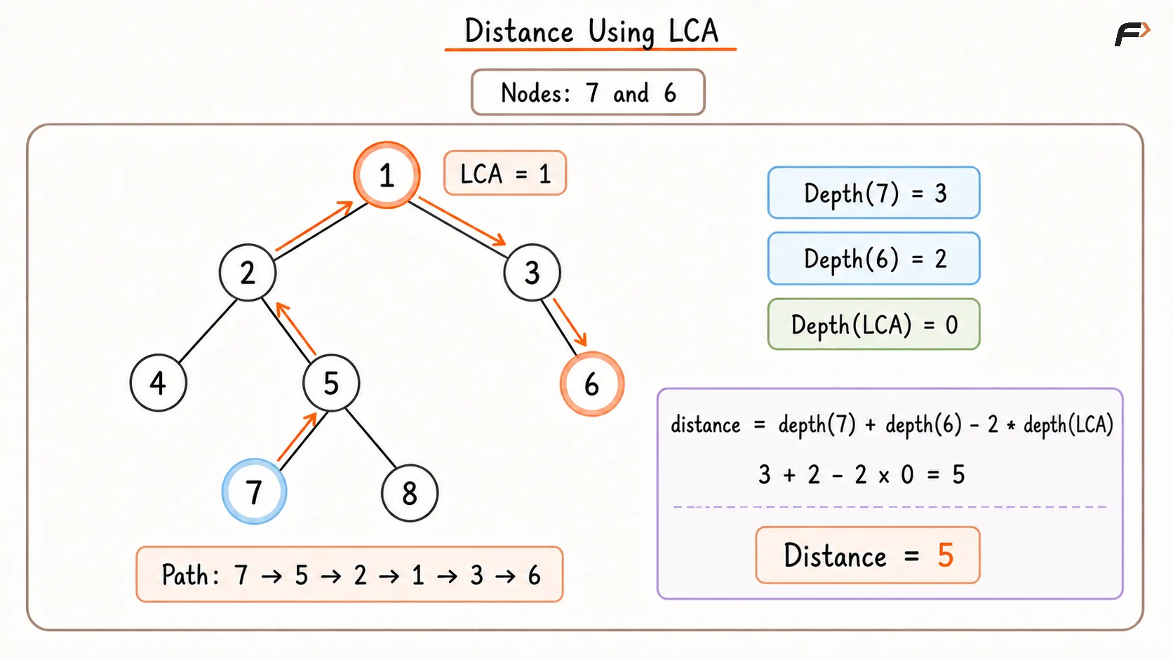
Distance Using LCA.png
Parent Mapping and LCA Comparison
Parent Mapping with BFS | Depth and LCA |
|---|---|
Useful for traversal outward from a target | Useful for direct distance calculations |
Naturally finds all nodes at distance | Naturally finds distance between two nodes |
Requires parent and visited structures | Requires depths and an LCA method |
Takes | Can support repeated queries with advanced preprocessing |
Models the tree as an undirected graph | Uses ancestor relationships |
The correct technique depends on whether the problem asks for nodes at a distance, the distance value itself, or many repeated distance queries.
Applications
Parent and distance concepts are used in:
Nodes at distance
KBurning tree problems
Infection-spread simulations
Finding the nearest leaf
Calculating distance between two nodes
Lowest Common Ancestor problems
Finding ancestors of a target
Rerooting a tree
Graph traversal on tree structures
Finding the farthest node or tree diameter
Common Mistakes
Counting nodes instead of edges while calculating distance.
Assuming the distance between two nodes is the difference between their depths.
Forgetting to create parent relationships before moving upward.
Traversing through parent links without a visited structure.
Marking nodes visited only after removal from the queue, allowing duplicate insertions.
Forgetting that the root has no parent.
Expanding one extra BFS level after reaching distance
K.Returning all visited nodes instead of only the current distance frontier.
Using node values as map keys when duplicate values are possible.
Assuming the order of nodes at distance
Kis automatically sorted.Applying the LCA distance formula with node-based depth in one place and edge-based depth in another.
Forgetting that a target leaf can still reach other branches through its ancestors.
FAQs
Q1. Why is a visited structure required after adding parent links?
Parent links make every edge traversable in both directions. Without visited tracking, traversal can repeatedly move from a child to its parent and back to the same child.
Q2. Is a parent mapping always necessary for distance problems?
No. Recursive distance calculations and LCA-based methods can avoid an explicit parent map. Parent mapping is especially convenient when BFS must begin from an arbitrary target and move in all three directions.
Q3. Can the distance between two nodes be calculated by subtracting their depths?
Only when one node is an ancestor of the other. In the general case, use their LCA: Depth(U) + Depth(V) - 2 × Depth(LCA).
Q4. How should duplicate node values be handled?
Use node references or unique identifiers as keys in parent and visited structures. A value alone may refer to more than one node and make the target ambiguous.
Q5. How can repeated distance queries on the same tree be optimized?
Preprocess node depths and ancestor information using techniques such as binary lifting. This allows LCA, and therefore distance, to be answered much faster than traversing the complete tree for every query.
Be the first to add a comment.