Complete Binary Tree Optimization – Introduction
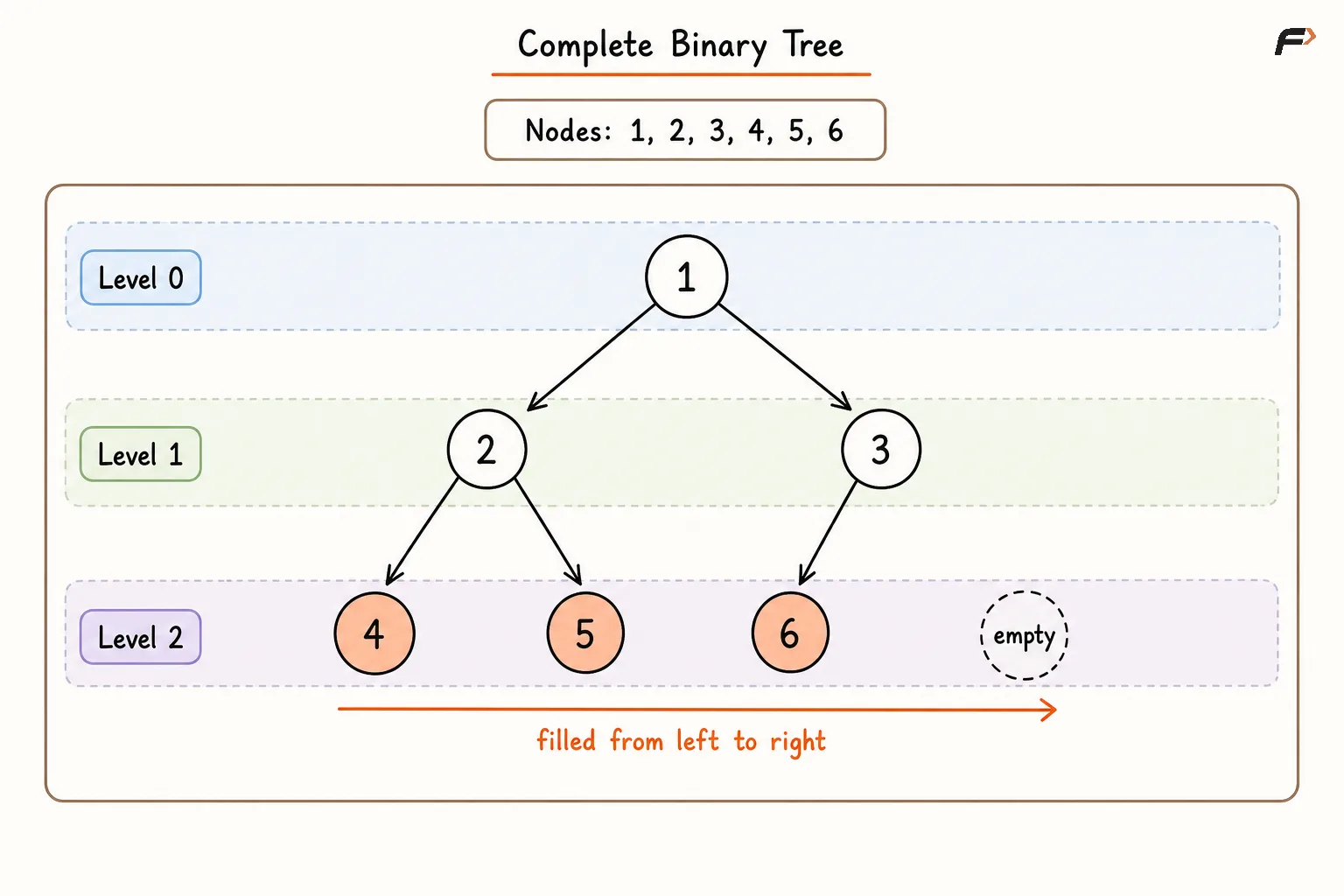
A complete binary tree is a binary tree in which:
Every level is completely filled except possibly the last level.
Nodes in the last level are placed as far left as possible.
Consider a tree containing six nodes:
Node
1is the root.Nodes
2and3are its children.Nodes
4and5are the children of2.Node
6is the left child of3.
Its levels are:
Level | Nodes |
|---|---|
|
|
|
|
|
|
The final level is incomplete, but its nodes occupy the leftmost available positions. Therefore, the tree is complete.
This predictable structure supports optimizations that are not valid for an arbitrary binary tree.
It allows us to:
Count nodes without visiting every node
Represent the tree compactly using an array
Search the final level using binary search
Locate parent and child positions using indices
Identify perfect subtrees through their extreme heights
Find insertion positions without a complete level-order scan when additional size information is available
Complete Binary Tree.png
Complete, Full, and Perfect Binary Trees
These terms describe different structural properties.
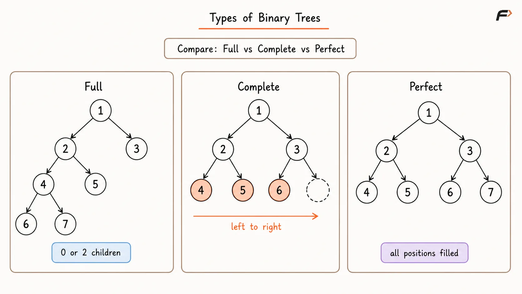
Tree Type | Condition |
|---|---|
Full Binary Tree | Every node has either zero or two children |
Complete Binary Tree | Every level except possibly the last is full, and the last level is filled from left to right |
Perfect Binary Tree | Every level is completely filled |
A perfect binary tree is both full and complete.
A complete binary tree does not need to be full. In the introductory example, node 3 has only a left child, so the tree is complete but not full.
A full tree does not need to be complete because its leaf nodes may appear at irregular positions or levels.
Types of Binary Trees.png
Structural Properties of a Complete Binary Tree
The usefulness of a complete binary tree comes from several guarantees.
All Higher Levels Are Full
If the tree has H levels, every level from 0 through H - 2 is completely filled.
Only level H - 1 may be incomplete.
The Last Level Is Left-Packed
If a position in the final level is empty, every position to its right must also be empty.
Therefore, the final level has a pattern similar to:
Occupied, Occupied, Occupied, Empty, Empty
It cannot have:
Occupied, Empty, Occupied
This monotonic occupied-to-empty pattern makes binary search possible.
Height Remains Logarithmic
A complete binary tree containing N nodes has:
H = floor(log₂ N) + 1
levels when N > 0.
Therefore:
H = O(log N)
Number of Nodes Above the Final Level
If the tree has H levels, the first H - 1 levels contain:
2ᴴ⁻¹ - 1
nodes.
Maximum Positions in the Final Level
The final level can contain at most:
2ᴴ⁻¹
nodes.
For a three-level tree:
Nodes above the last level:
2² - 1 = 3Maximum final-level positions:
2² = 4
Array Representation
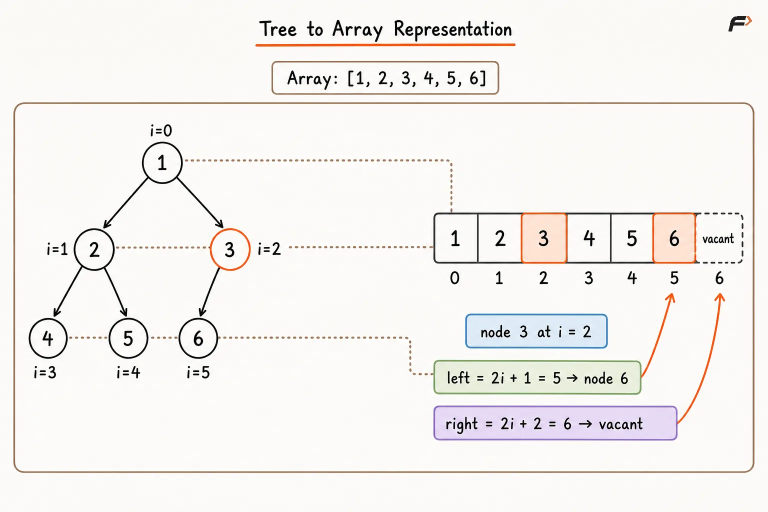
A complete binary tree can be stored compactly in an array without gaps.
Using zero-based indexing, for a node at index i:
Left Child Index = 2i + 1
Right Child Index = 2i + 2
For a non-root node:
Parent Index = floor((i - 1) / 2)
The introductory tree is represented as:
[1, 2, 3, 4, 5, 6]
Its relationships are:
Node | Index | Left Child Index | Right Child Index |
|---|---|---|---|
|
|
|
|
|
|
|
|
|
|
|
|
Index 5 contains node 6, while index 6 lies outside the current array and represents the next available position.
This compact representation is one reason binary heaps use complete binary trees.
Tree to Array Representation.png
Why Does Completeness Enable Optimization?
In an arbitrary binary tree:
Missing nodes can appear anywhere.
Equal extreme heights do not prove that every internal position exists.
The last level does not have a searchable occupied-to-empty pattern.
Array representation may contain large gaps.
In a complete binary tree:
All uncertainty is limited to the final level.
Existing final-level nodes form one continuous prefix.
Many subtrees are perfect.
Height is logarithmic.
Index-based paths can be derived from binary representations.
These guarantees allow entire perfect subtrees to be counted mathematically instead of node by node.
Counting Nodes in a Complete Binary Tree
Given the root of a complete binary tree, determine its total number of nodes.
For the introductory tree:
Node Count = 6
A normal traversal visits all six nodes. However, the complete-tree property allows the count to be calculated more efficiently.
Approach 1
Intuition
The straightforward method recursively counts every node.
For each non-empty node:
Count = 1 + Count(left subtree) + Count(right subtree)
This approach works for every binary tree and does not rely on completeness.
Algorithm
Return
0when the current node isNULL.Recursively count the nodes in the left subtree.
Recursively count the nodes in the right subtree.
Add
1for the current node.Return the combined count.
Time Complexity: O(N) because every node is visited.
Space Complexity: O(H) due to the recursion stack.
Since a complete binary tree has logarithmic height:
Space Complexity = O(log N)
Approach 2
Intuition
A perfect binary tree with H levels contains:
2ᴴ - 1
nodes.
Therefore, if a subtree is perfect, its node count can be calculated immediately without traversing its internal nodes.
For a subtree of a complete binary tree:
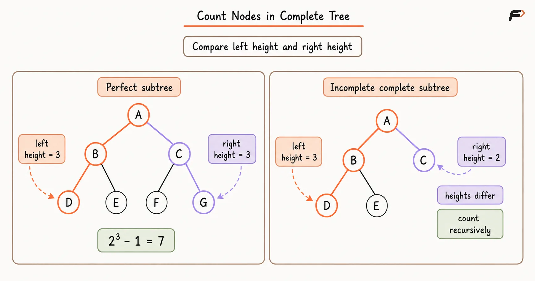
Follow left-child references to calculate its leftmost height.
Follow right-child references to calculate its rightmost height.
If both heights are equal, the subtree is perfect.
Otherwise, recursively count its left and right subtrees.
The equality test is valid because the input is guaranteed to be complete.
Measuring the Extreme Heights
In this article, height for this optimization is measured as the number of nodes on the path.
Therefore:
An empty subtree has height
0.A leaf has height
1.A perfect three-level tree has height
3.
Leftmost Height
Begin at the subtree root and repeatedly move to the left child until NULL is reached.
Rightmost Height
Begin at the subtree root and repeatedly move to the right child until NULL is reached.
If:
Leftmost Height = Rightmost Height = H
then the subtree contains:
2ᴴ - 1
nodes.
Count Nodes in Complete Tree comapre left and right ht .png
Algorithm
Return
0when the current subtree is empty.Calculate its leftmost height by following left-child references.
Calculate its rightmost height by following right-child references.
If the two heights are equal, return
2ᴴ - 1because the complete subtree must be perfect.Otherwise, recursively count the left and right subtrees.
Add
1for the current root and return the total.
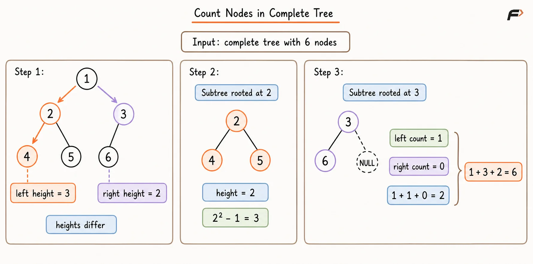
Dry Run
Consider the complete tree containing nodes 1 through 6.
Check the Subtree Rooted at 1
Leftmost path:
1 → 2 → 4
Leftmost Height = 3
Rightmost path:
1 → 3
Rightmost Height = 2
The heights are different, so the complete tree is not perfect.
Continue with its subtrees.
Check the Subtree Rooted at 2
Leftmost path:
2 → 4
Leftmost Height = 2
Rightmost path:
2 → 5
Rightmost Height = 2
The heights are equal, so this subtree is perfect.
Its node count is:
2² - 1 = 3
There is no need to visit nodes 4 and 5 individually.
Check the Subtree Rooted at 3
Leftmost path:
3 → 6
Leftmost Height = 2
Rightmost path:
3
Rightmost Height = 1
The heights are different.
Its left subtree rooted at 6 is perfect and contains:
2¹ - 1 = 1
Its right subtree is empty and contains:
0
Therefore, the subtree rooted at 3 contains:
1 + 1 + 0 = 2
Final Count
Root + Left Subtree + Right Subtree
= 1 + 3 + 2
= 6
Count Nodes in Complete Tree.png
Why Does the Height-Based Approach Work?
A perfect subtree can be counted directly because every position across all its levels is occupied.
Within a complete tree:
Equal leftmost and rightmost heights prove that the current subtree reaches the same deepest level on both extremes.
Completeness guarantees that no internal position between those extremes is missing.
Therefore, every level of that subtree is full.
When the heights differ, the current subtree is complete but not perfect. One of its child subtrees is perfect, while the other child contains the remaining incomplete portion.
Although the algorithm calls the counting function for both children, both calls do not continue recursively through all their descendants.
Because one child subtree is always perfect, the algorithm evaluates it in O(log N) and only recurses down the remaining non-perfect child.
The perfect child requires only its leftmost and rightmost height calculations. Once those heights are equal, its node count is returned directly using:
2ᴴ - 1
Therefore, the recursion follows only one chain of non-perfect subtrees instead of branching into two complete recursive searches.
Complexity Analysis
At a subtree with height H, calculating its leftmost and rightmost heights requires:
O(H)
One child subtree is perfect and is counted after its extreme heights are evaluated. Only the other, non-perfect child continues the recursive chain.
Therefore, the recurrence is:
T(H) = T(H - 1) + O(H)
It is not:
T(H) = 2T(H - 1)
Summing the height calculations across the recursive chain gives:
H + (H - 1) + (H - 2) + ... + 1 = O(H²)
A complete binary tree has:
H = O(log N)
Therefore:
Time Complexity: O(log² N)
The recursion follows at most one non-perfect child at each level, so its maximum depth is:
O(H) = O(log N)
Space Complexity: O(log N)
This is why the recursive method does not expand into an O(N) traversal.
Approach 3
Intuition
All levels above the final level are completely filled. Therefore, their node count is already known.
Only the number of existing nodes in the final level must be determined.
For a tree with H levels:
Nodes above final level = 2ᴴ⁻¹ - 1
The final level contains up to:
2ᴴ⁻¹
possible positions.
Because the existing positions form a continuous prefix followed by empty positions, binary search can find the boundary between them.
Indexing the Final Level
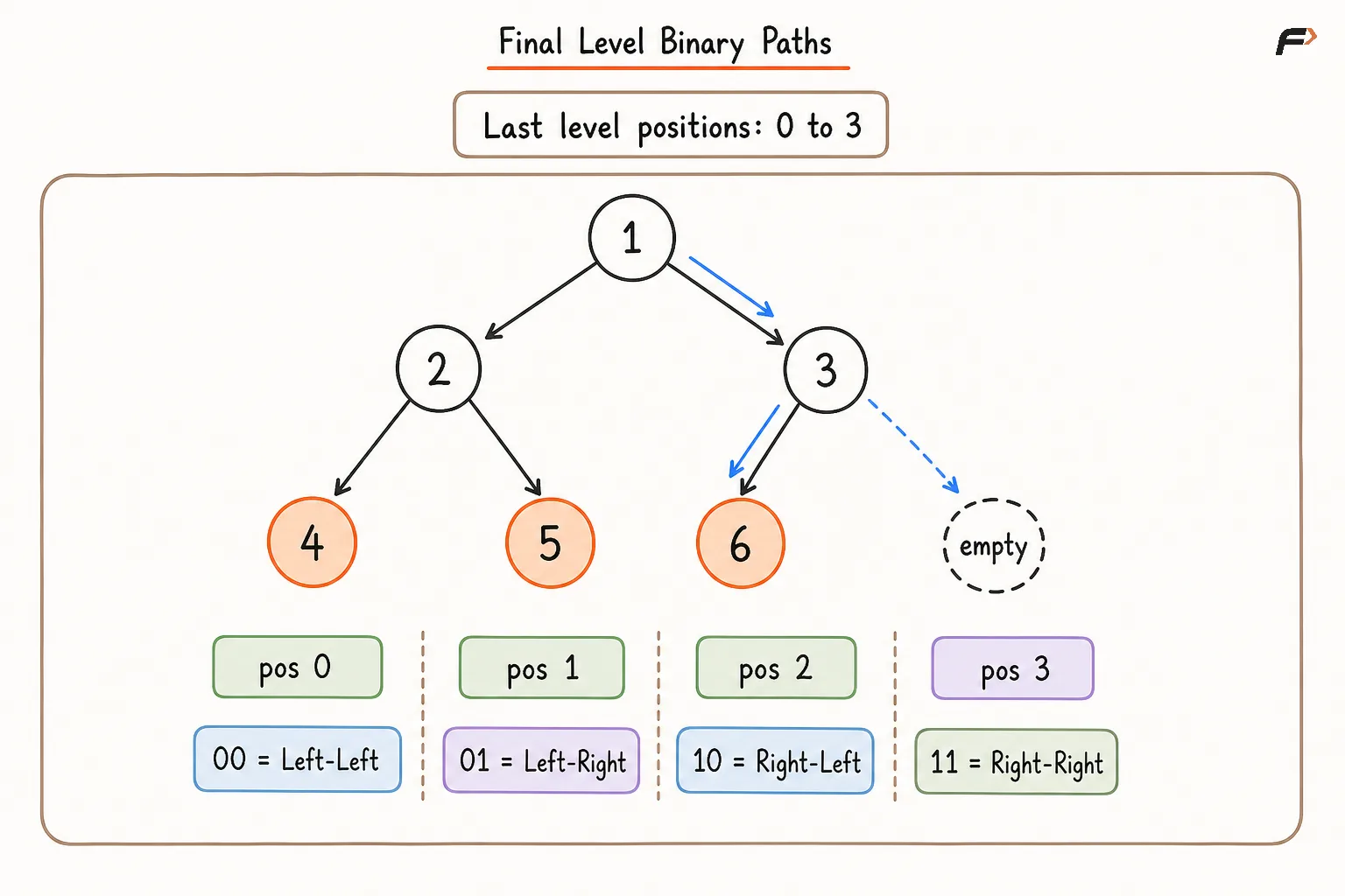
For the three-level example, the final level contains four possible positions:
Final-Level Index | Root-to-Position Path | State |
|---|---|---|
| Left → Left | Node |
| Left → Right | Node |
| Right → Left | Node |
| Right → Right | Empty |
The existence pattern is:
Exists, Exists, Exists, Missing
This monotonic pattern allows binary search.
The binary representation of a final-level index can also describe its path:
0bit means move left.1bit means move right.
For two path decisions:
00means Left → Left.01means Left → Right.10means Right → Left.11means Right → Right.
Final Level Binary Paths.png
Checking Whether a Final-Level Node Exists
A final-level index contains exactly H - 1 path decisions because the path begins at the root and moves through one edge for every remaining level.
Represent the index using H - 1 bits:
0means move to the left child.1means move to the right child.
For a zero-based step value from 0 to H - 2, calculate the next direction using:
directionBit = (index >> (H - 2 - step)) & 1
Here:
H - 2 - stepidentifies the bit required for the current level.Right shift moves that bit to the least significant position.
& 1extracts its value.If
directionBit = 0, move left.If
directionBit = 1, move right.
For example, let:
H = 3
index = 2 = 10₂
There are two path decisions.
At step = 0:
(2 >> (3 - 2 - 0)) & 1
= (2 >> 1) & 1
= 1
Therefore, move right.
At step = 1:
(2 >> (3 - 2 - 1)) & 1
= (2 >> 0) & 1
= 0
Therefore, move left.
Thus, final-level index 2 represents:
Right → Left
If the required child becomes NULL at any step, the final-level position does not exist. If all H - 1 decisions are completed at a valid node, the position exists.
Each existence check follows one root-to-final-level path and takes:
O(log N)
Algorithm
Return
0if the tree is empty.Calculate the number of levels
Hby following the leftmost path.Count the nodes above the final level using
2ᴴ⁻¹ - 1.Binary search the final-level indices from
0to2ᴴ⁻¹ - 1.For each middle index, begin at the root and process steps from
0toH - 2.At every step, calculate
(index >> (H - 2 - step)) & 1.Move to the left child when the extracted bit is
0; otherwise, move to the right child.Treat the position as missing if the required node becomes
NULL.Use the existence result to continue binary search toward the last occupied final-level position.
Add the number of existing final-level nodes to the known count of nodes above that level.
Dry Run
For the six-node tree:
H = 3
Nodes above the last level:
2² - 1 = 3
Possible positions in the last level:
2² = 4
Their states are:
[Exists, Exists, Exists, Missing]
Binary search locates the final existing position at index 2.
Therefore, the number of existing nodes in the final level is:
3
Total nodes:
3 + 3 = 6
Complexity Analysis
The final level contains O(N) possible positions, so binary search performs:
O(log N)
existence checks.
Each existence check follows a path of length:
O(log N)
Therefore:
Time Complexity: O(log² N)
If path checks are performed iteratively:
Auxiliary Space Complexity: O(1)
The tree itself is not modified during this process.
Comparison of the Approaches
Approach | Time Complexity | Auxiliary Space | Main Idea |
|---|---|---|---|
Approach 1 |
|
| Visit and count every node |
Approach 2 |
|
| Count perfect subtrees directly |
Approach 3 |
|
| Binary search the final level |
Approach 2 is often easier to implement recursively.
Approach 3 makes the left-packed final-level property more explicit and can avoid recursive stack space.
Other Complete-Tree Optimizations
Efficient Heap Representation
A complete tree can be stored without gaps in an array. This enables direct parent and child index calculations and efficient heap operations.
Finding the Next Insertion Position
If the current node count is known, the next node receives conceptual array index N.
The binary representation of this index can be used to derive the path from the root to its parent.
This can locate the insertion position in:
O(log N)
time instead of scanning the tree level by level.
Compact Memory Usage
Complete trees avoid the large gaps that a sparse tree would create in array representation.
Predictable Height
Since height remains logarithmic, upward and downward heap operations require at most:
O(log N)
steps.
When Can These Optimizations Be Used?
Use complete-tree optimizations only when the problem guarantees that the tree is complete or when that property has already been established.
Suitable clues include:
“The given tree is complete.”
“All levels except possibly the last are full.”
“The last level is filled from left to right.”
“Count nodes in a complete binary tree.”
“The tree is represented as a binary heap.”
If completeness is not guaranteed, use a general traversal or first verify the structure.
Verifying completeness takes O(N) time, which may remove the advantage of an O(log² N) counting method for a single query.
Important Edge Cases
Empty Tree
Node Count = 0
Its number of levels is treated as 0.
Single-Node Tree
Both extreme heights are 1.
Node Count = 2¹ - 1 = 1
Perfect Tree
The root’s leftmost and rightmost heights are equal, so the count is returned immediately.
Final Level Contains One Node
The complete-tree property places that node at the leftmost final-level position.
Large Height
Expressions involving powers of two may overflow a narrow integer type. A sufficiently wide type should be used when calculating:
2ᴴ
Common Mistakes
Confusing complete, full, and perfect binary trees.
Assuming a complete tree must have every level completely filled.
Applying the optimization when completeness is not guaranteed.
Assuming equal extreme heights prove perfection in an arbitrary binary tree.
Mixing edge-based height with level-based height.
Using
2ᴴinstead of2ᴴ - 1for the number of nodes in a perfect subtree.Forgetting that only the final level may be incomplete.
Treating final-level occupancy as non-monotonic.
Using an incorrect left-right path for a final-level index.
Counting final-level positions instead of existing nodes.
Forgetting the empty-tree and single-node cases.
Overflowing a narrow integer while calculating a power of two.
Claiming the height-based method is
O(log N)even though heights are recalculated across recursive levels.Assuming node values or Binary Search Tree ordering are relevant to these optimizations.
FAQs
Q1. Why does equal leftmost and rightmost height prove that a complete subtree is perfect?
Completeness guarantees that final-level nodes occupy a continuous prefix. If both extremes reach the same deepest level, the rightmost possible position also exists, so every position between the two extremes must be filled.
Q2. Why is the optimized counting complexity O(log² N) instead of O(log N)?
The algorithm processes up to O(log N) incomplete levels, and height or existence checks at those levels can each take O(log N) time. Their combination gives O(log² N).
Q3. Which optimized counting method should be preferred?
Perfect-subtree detection is usually simpler and directly follows the recursive structure. Last-level binary search provides the same asymptotic time and can use O(1) auxiliary space when implemented iteratively.
Q4. What should be done if the tree is not guaranteed to be complete?
Use a normal O(N) traversal. Checking completeness first also takes O(N), so it generally does not improve a single node-count query.
Q5. How can knowing the current node count optimize insertion?
The next node has conceptual array index N. The bits of that index identify the left-right path to its parent, allowing the insertion position to be located in O(log N) time when the tree’s size is already known.
Be the first to add a comment.