Level Order Traversal of a Binary Tree Using BFS

Introduction to BFS and Level Order Traversal

Breadth-First Search, or BFS, is a traversal technique that visits nodes according to their distance from the starting node.

In a binary tree, BFS begins at the root and processes the tree one level at a time:

• Visit the root.

• Visit every node at the next level.

• Continue moving downward until all nodes are processed.

For binary trees, BFS is commonly called level order traversal.

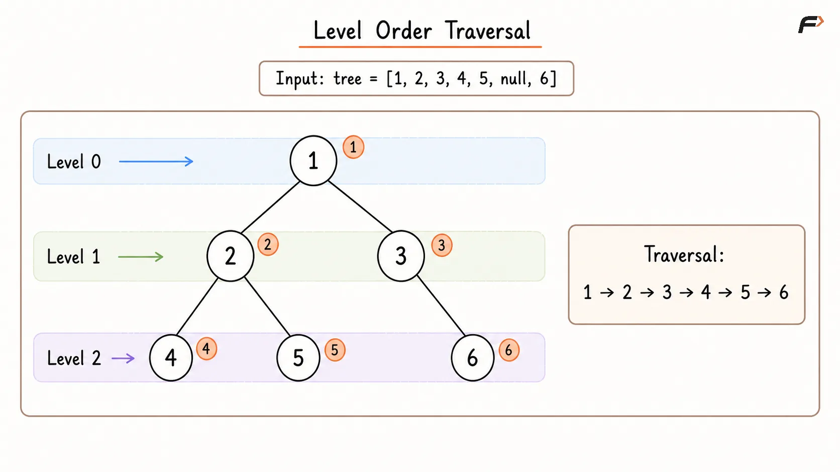
Consider a binary tree with the following relationships:

• Node 1 is the root.

• Nodes 2 and 3 are the children of 1.

• Nodes 4 and 5 are the children of 2.

• Node 6 is the right child of 3.

The nodes are arranged by level as follows:

• Level 0: 1

• Level 1: 2, 3

• Level 2: 4, 5, 6

Therefore, the level order traversal is:

1, 2, 3, 4, 5, 6

How Does BFS Work?

BFS processes nodes in the order in which they are discovered.

When a node is visited:

• Its value is processed.

• Its left child is scheduled for future processing.

• Its right child is scheduled for future processing.

• The traversal then moves to the earliest node that is still waiting.

This order is maintained using a queue.

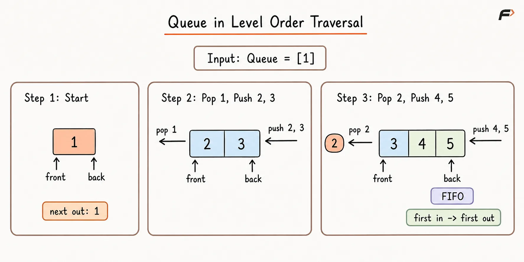
A queue follows the First In, First Out, or FIFO, principle:

• Nodes are inserted at the back.

• Nodes are removed from the front.

• A node discovered earlier is processed earlier.

Because all nodes of one level are discovered before the nodes of the next level, the queue naturally maintains level order.

Why Is a Queue Used?

Suppose the root’s children are discovered in the order:

2, 3

Both nodes must be processed before their children.

After processing 2, its children 4 and 5 are added after 3:

3, 4, 5

Therefore, node 3 is still processed before nodes 4 and 5.

This is exactly the order maintained by a queue.

A stack would process the most recently added node first, causing the traversal to move deeper into one branch. That behaviour corresponds to DFS, not BFS.

The BFS Mental Model

A useful way to understand level order traversal is:

Remove one node from the front, process it, and place its existing children at the back.

The queue always contains the nodes that have been discovered but not yet processed.

At any moment:

• Nodes near the front were discovered earlier.

• Nodes near the back were discovered later.

• Children are processed only after the nodes of the previous level.

The main BFS cycle is:

1. Remove the front node.

2. Process its value.

3. Add its left child if it exists.

4. Add its right child if it exists.

5. Repeat until the queue becomes empty.

Basic Level Order Traversal

Given the root of a binary tree, return its nodes in level order from left to right.

Algorithm

• Check whether the root is NULL; if so, the traversal is empty.

• Create a queue and place the root inside it because traversal begins from the first level.

• Remove the node at the front of the queue and process its value.

• Add its left child followed by its right child whenever those children exist.

• Continue removing and adding nodes until the queue becomes empty.

• Return the values in the order in which the nodes were processed.

Time Complexity: O(N) because every node is inserted into and removed from the queue once.

Space Complexity: O(W), where W is the maximum number of nodes present at any level.

Dry Run of Level Order Traversal

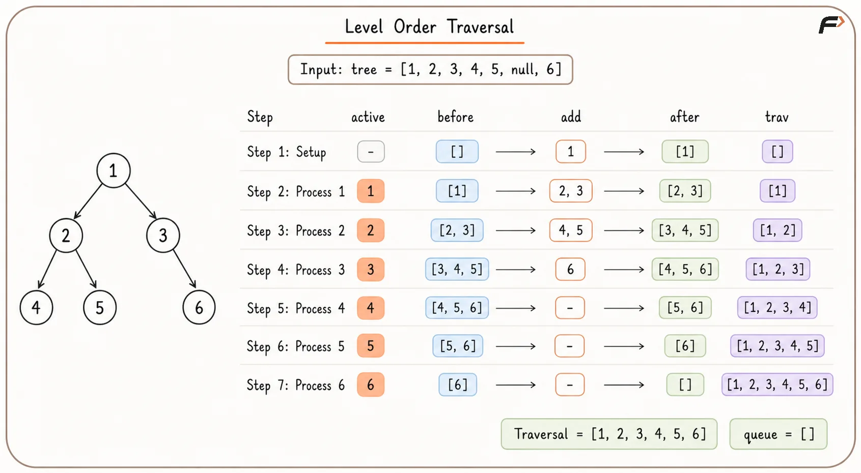
Consider the earlier tree.

Initial state:

Queue = [1]

Traversal = []

Step 1: Process Node 1

Remove 1 from the queue:

Traversal = [1]

Add its children 2 and 3:

Queue = [2, 3]

Step 2: Process Node 2

Remove 2:

Traversal = [1, 2]

Add its children 4 and 5:

Queue = [3, 4, 5]

Step 3: Process Node 3

Remove 3:

Traversal = [1, 2, 3]

Node 3 has no left child, so add only its right child 6:

Queue = [4, 5, 6]

Step 4: Process Node 4

Remove 4:

Traversal = [1, 2, 3, 4]

Node 4 has no children:

Queue = [5, 6]

Step 5: Process Node 5

Remove 5:

Traversal = [1, 2, 3, 4, 5]

Node 5 has no children:

Queue = [6]

Step 6: Process Node 6

Remove 6:

Traversal = [1, 2, 3, 4, 5, 6]

Node 6 has no children:

Queue = []

The queue is empty, so traversal is complete.

Final level order:

1, 2, 3, 4, 5, 6

Returning Nodes Level by Level

Sometimes the output must preserve separate levels instead of returning one flat sequence.

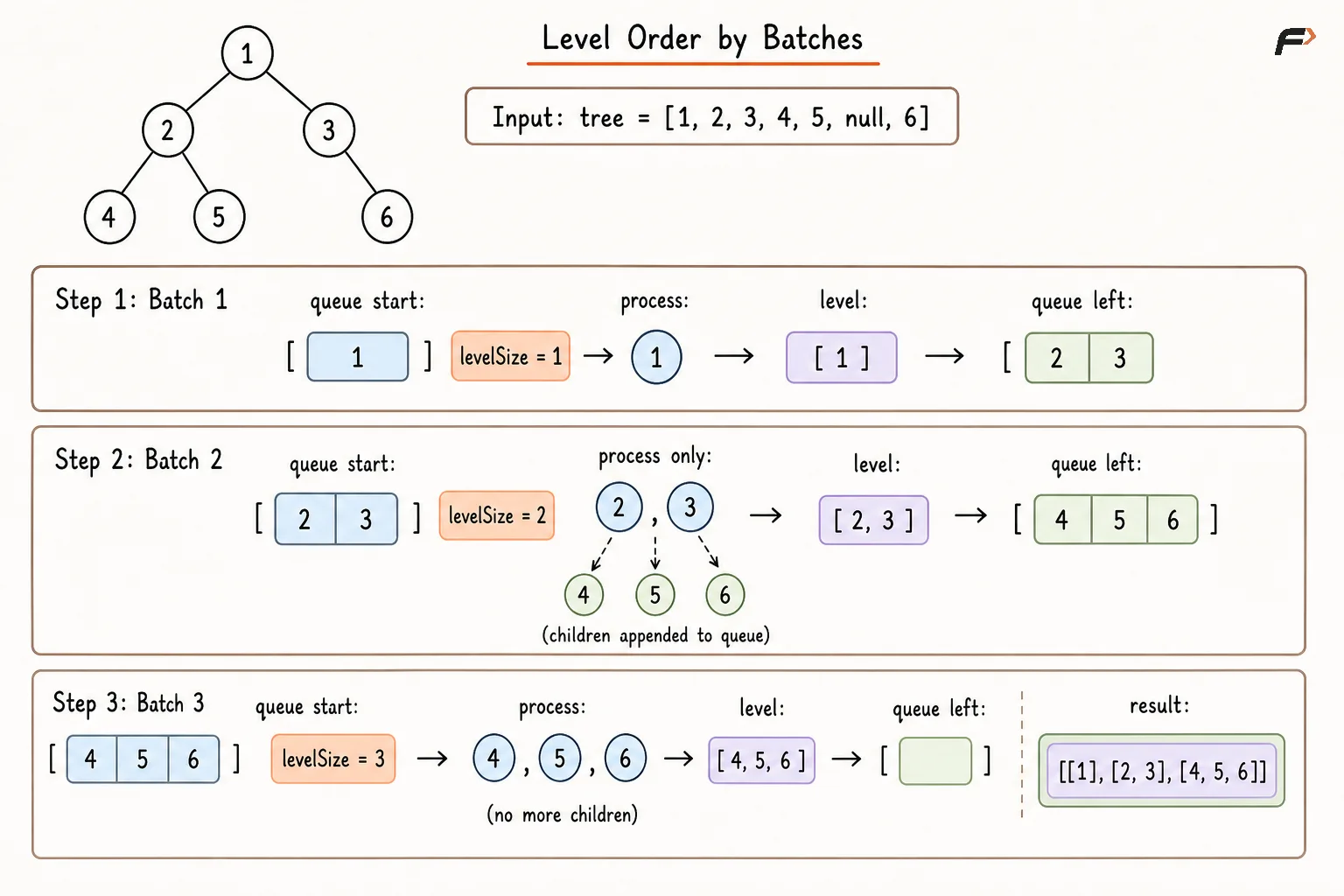
For the example tree, the required result is:

[[1], [2, 3], [4, 5, 6]]

To separate levels, record the queue size before processing the current level.

If the queue currently contains:

[2, 3]

then the current level contains exactly two nodes.

Process exactly those two nodes, even though their children are being added to the queue during the same process.

After processing both nodes:

• The current level is complete.

• The remaining queue contains only nodes from the next level.

Why Must the Queue Size Be Recorded First?

The queue changes while a level is being processed.

Suppose the current queue is:

[2, 3]

Its initial size is:

2

While processing these two nodes, their children are added:

• Processing 2 adds 4 and 5.

• Processing 3 adds 6.

The queue becomes:

[4, 5, 6]

These three nodes belong to the next level and must not be processed as part of the current level.

Therefore, save:

levelSize = current queue size

before processing the level.

Algorithm

• Place the root into the queue if it exists.

• Continue while the queue is not empty.

• Record the current queue size as the number of nodes in the active level.

• Process exactly that many nodes and store their values together.

• Add the children of those nodes to the queue for the next level.

• Add the completed level to the final result.

Time Complexity: O(N)

Space Complexity: O(W) auxiliary space, excluding the returned level lists.

Understanding the Space Complexity

The space used by level order traversal has two separate parts:

• Auxiliary queue memory: The queue temporarily stores nodes that have been discovered but not yet processed.

• Output storage memory: The returned traversal stores the value of every node.

These two types of memory should be reported separately.

Auxiliary Queue Memory

The queue does not necessarily store all N nodes simultaneously. Its maximum size depends on the tree’s maximum width.

Therefore:

Auxiliary Queue Space = O(W)

where W is the maximum number of nodes present at any level.

This is the working memory required by the BFS algorithm and excludes the returned traversal.

Output Storage Memory

If the traversal values are stored and returned, every node appears once in the output.

Therefore:

Output Space = O(N)

This memory is required to hold the answer and is generally excluded when reporting auxiliary space.

If output storage is included in the total space calculation:

Total Space = O(W + N)

Since W ≤ N, this simplifies to:

Total Space = O(N)

Skewed Tree

A skewed tree contains only one node at each level, so:

W = 1

Therefore:

• Auxiliary queue space: O(1)

• Output storage: O(N)

• Total space including output: O(N)

Perfect Binary Tree

The last level of a perfect binary tree contains approximately half of all its nodes, so:

W = O(N)

Therefore:

• Auxiliary queue space: O(N)

• Output storage: O(N)

• Total space including output: O(N)

Thus, the standard BFS space complexity is reported as O(W) auxiliary space. If the returned traversal is also counted, the complete space usage is O(N).

Common Variations of Level Order Traversal

The same queue-based framework can solve many binary-tree problems.

1. Reverse Level Order

Process nodes from top to bottom using BFS, then reverse the collected levels.

Example:

[[4, 5, 6], [2, 3], [1]]

2. Zigzag Level Order

Alternate the output direction at each level:

• First level from left to right

• Second level from right to left

• Third level from left to right

For the example:

[[1], [3, 2], [4, 5, 6]]

3. Left View

Record the first node processed at every level.

For the example:

[1, 2, 4]

4. Right View

Record the last node processed at every level.

For the example:

[1, 3, 6]

5. Level Sum or Average

Calculate the sum or average of all node values within each level.

6. Maximum Width

Use the number of nodes or positional indices at each level to calculate the tree’s width, depending on the problem’s definition.

7. Minimum Depth

The first leaf reached by BFS has the minimum depth because BFS processes nodes in increasing order of their distance from the root.

8. Connecting Nodes at the Same Level

All nodes in the current queue batch belong to the same level, allowing neighbouring nodes to be linked or compared.

Finding Minimum Depth Using BFS

The minimum depth is the number of nodes or edges on the shortest path from the root to a leaf, depending on the convention used.

BFS explores the tree level by level. Therefore, the first leaf encountered belongs to the shallowest level containing any leaf.

The traversal can stop immediately after finding that leaf.

A leaf must have:

• No left child

• No right child

A node with only one missing child is not a leaf.

This early termination can avoid exploring deeper levels that cannot contain a shorter answer.

BFS and Shortest Paths

In an unweighted graph, BFS finds the shortest path measured by the number of edges.

This works because BFS processes nodes in increasing order of distance from the source:

• Source at distance 0

• Its neighbours at distance 1

• Their unvisited neighbours at distance 2

• The process continues outward

A binary tree is already connected without cycles, so level order traversal does not normally require a visited structure.

A general graph may contain:

• Cycles

• Multiple paths to the same node

• Disconnected components

Therefore, graph BFS must track visited nodes.

BFS on Trees and Graphs

If a tree representation contains parent references as well as child references, traversal can move back to an already processed node. In that case, a visited structure or previous-node reference is required.

BFS and DFS Comparison

Neither traversal is universally better. The correct choice depends on whether the problem is based on levels, distance, paths, or subtree information.

When Should BFS Be Used?

Consider BFS when the problem asks for:

• Level order traversal

• Nodes grouped by depth

• Minimum depth of a tree

• Left or right view

• Zigzag traversal

• Average or sum of each level

• Maximum number of nodes at a level

• Nearest node satisfying a condition

• Shortest path in an unweighted graph

• Connections between nodes at the same level

A strong recognition clue is that the answer depends on processing nearer nodes before deeper nodes.

Advantages of BFS

• It naturally processes nodes by level.

• It finds the nearest valid node first.

• It supports shortest-path calculations in unweighted graphs.

• It avoids recursion-depth problems.

• It can stop early when the first valid level is reached.

• It provides a reusable framework for many level-based tree problems.

Limitations of BFS

• A wide tree may require O(N) queue space.

• It does not naturally calculate values that depend on completed subtrees.

• Level separation requires careful queue-size handling.

• Graph BFS needs a visited structure.

• It may explore many nodes before reaching a deep target.

• It does not provide inorder, preorder, or postorder sequences.

Common Mistakes

• Forgetting to handle a NULL root before placing it in the queue.

• Using a stack instead of a queue.

• Adding right children before left children when left-to-right order is required.

• Adding NULL children unnecessarily.

• Recording the queue size repeatedly while processing the same level.

• Processing newly added children as part of the current level.

• Forgetting that queue space depends on maximum width, not height.

• Marking graph nodes as visited too late and inserting them multiple times.

• Treating a node with one missing child as a leaf.

• Assuming BFS always requires O(N) space without stating the tighter O(W) bound.

• Including the returned traversal inside auxiliary space without stating the convention.

• Using BFS for a subtree-dependent calculation that is more naturally solved with postorder DFS.

FAQs

Q1. Why is a queue necessary for BFS instead of a stack?

A queue processes the earliest discovered node first, preserving level order. A stack processes the most recently discovered node first and therefore moves deeper into one branch, producing DFS-like behaviour.

Q2. How are separate levels identified during level order traversal?

Record the queue size before processing a level. That size represents exactly the nodes currently belonging to the active level. Children added during processing remain in the queue for the next level.

Q3. Why is the auxiliary space complexity O(W) rather than O(H)?

The queue may store many nodes from the same level simultaneously, so its maximum size depends on tree width. DFS stores an active root-to-node path, so its recursive space depends on height.

Q4. Why does BFS find the minimum depth or shortest unweighted path?

BFS processes nodes in increasing order of their distance from the source. Therefore, the first valid target or leaf reached cannot have another undiscovered path with fewer edges.

Q5. Why is a visited structure unnecessary for a normal binary tree but required for a graph?

A binary tree is acyclic, and every non-root node has one parent path, so a node is reached only once through child references. A graph may contain cycles and several paths to the same node, so visited tracking prevents repeated processing.