Matrix Traversal One Shot
What is a Matrix?
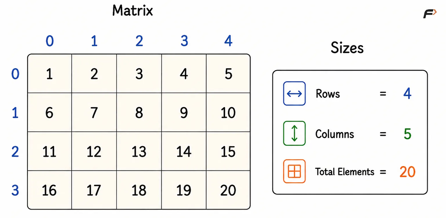
A matrix is a rectangular arrangement of values organized into rows and columns. Every value occupies a unique position identified by its row index and column index.
For example, consider the following matrix:
matrix
Think of a matrix as a classroom seating chart, a chessboard, a spreadsheet, or the pixels of an image, where every cell has a fixed location.
Why Are Matrices Used?
In programming, a matrix is stored as a two-dimensional array. The first index represents the row, and the second index represents the column. mat[row][col]
Examples: mat[0][0] = 1, mat[1][3] = 9
Matrices are widely used because they naturally represent structured data such as:
Grids and game boards
Tables and spreadsheets
Maps and mazes
Images (pixel matrices)
Dynamic Programming tables
Graph adjacency matrices
Scientific and mathematical computations
Understanding Matrix Indices
Every cell is uniquely identified by its (row, column) index.
           Column   Column   Column
             0        1        2
        ┌────────┬────────┬────────┐
Row 0   │ (0,0)  │ (0,1)  │ (0,2)  │
        ├────────┼────────┼────────┤
Row 1   │ (1,0)  │ (1,1)  │ (1,2)  │
        ├────────┼────────┼────────┤
Row 2   │ (2,0)  │ (2,1)  │ (2,2)  │
        └────────┴────────┴────────┘
For a matrix having N rows and M columns:
Row indices range from 0 to N − 1
Column indices range from 0 to M − 1
Principal and Secondary Diagonal
Diagonal traversal is commonly performed on square matrices, where the number of rows and columns is the same.
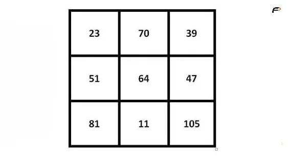
For the matrix:
matrix 1
Principal Diagonal (Main Diagonal)
The principal diagonal starts from the top-left corner and ends at the bottom-right corner.
Every element on this diagonal satisfies: row = column
Principal diagonal: 23 64 105
Secondary Diagonal (Anti-Diagonal)
The secondary diagonal starts from the top-right corner and ends at the bottom-left corner.
Every element on this diagonal satisfies: row + column = N − 1 (where N is the size of the square matrix.)
Secondary diagonal: 39 64 81
What is Matrix Traversal?
Matrix traversal means visiting every cell of a matrix in a specific order to process or access its values.
Depending on the problem, traversal can happen in different patterns.
Traversal Type | Visiting Order |
|---|---|
Row-wise | Left → Right for every row |
Column-wise | Top → Bottom for every column |
Main Diagonal | Top-left → Bottom-right |
Anti Diagonal | Top-right → Bottom-left |
Row-Wise Print in a Matrix
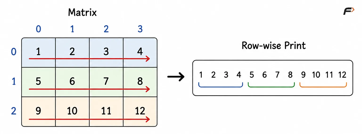
Given a matrix with N rows and M columns, print all elements row by row from left to right.
For a detailed explanation, see the original TUF blog:Row Wise Traversal
Example 1
Input: mat = [[1, 2, 3], [4, 5, 6]]
Output: 1 2 3 4 5 6
Explanation: First row prints as 1 2 3, followed by second row as 4 5 6.
Algorithm
Find the number of rows and columns in the matrix.
Traverse every row using an outer loop.
For each row, traverse all columns using an inner loop.
Print the current element.
Continue until all rows and columns have been processed.
row wise
Complexity Analysis
Time Complexity: O(N × M), every matrix cell is visited exactly once.
Space Complexity: O(1), only loop variables are used apart from output handling.
Column-Wise Print in a Matrix
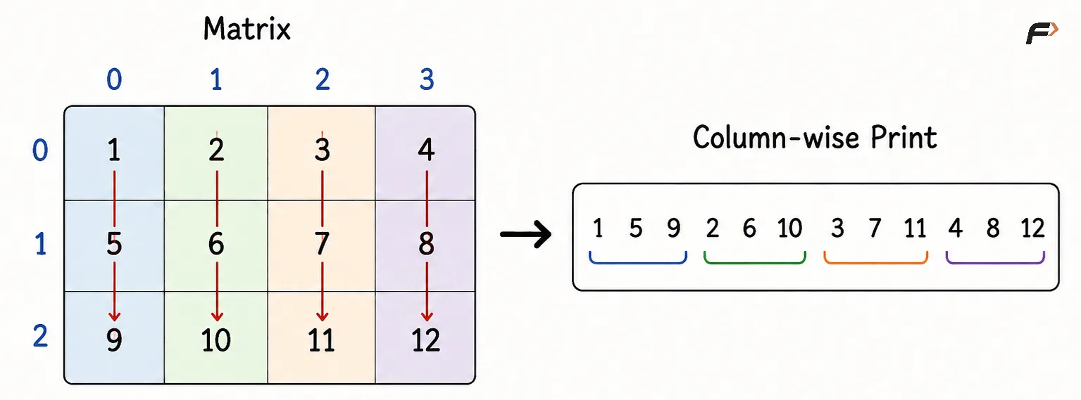
Given a matrix with N rows and M columns, print all elements column by column from top to bottom.
For a detailed explanation, see the original TUF blog: Column Wise Traversal
Example 1
Input: mat = [[1, 2, 3], [4, 5, 6]]
Output: 1 4 2 5 3 6
Explanation: First column prints as 1 4, followed by second column as 2 5, then third column as 3 6.
Algorithm
Find the number of rows and columns in the matrix.
Traverse every column using an outer loop.
For each column, traverse all rows using an inner loop.
Print the current element.
Continue until all rows and columns have been processed.
column wise
Complexity Analysis
Time Complexity: O(N × M), every matrix cell is visited exactly once.
Space Complexity: O(1), only loop variables are used apart from output handling.
Main Diagonal Print in a Matrix
Given a matrix with N rows and M columns, print all elements present on the main diagonal.
The main diagonal starts from the top-left cell and moves one step down and one step right at each move. Every selected cell has equal row index and column index.
For a detailed explanation, see the original TUF blog: Main Diagonal Traversal
Example 1
Input: mat = [[1, 2, 3], [4, 5, 6], [7, 8, 9]]
Output: 1 5 9
Explanation: Main diagonal cells are mat[0][0], mat[1][1], and mat[2][2].
Algorithm
Find the number of rows and columns in the matrix.
Compute the traversal limit as the smaller of the two dimensions.
Traverse the diagonal indices from
0tolimit - 1.Print the element at
mat[index][index].Continue until all main diagonal elements have been processed.
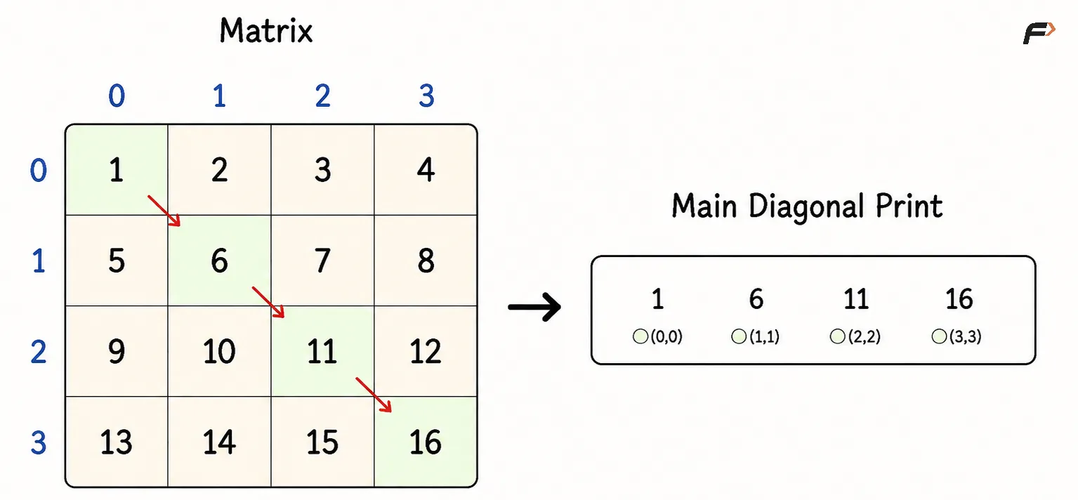
main diagonal
Complexity Analysis
Time Complexity: O(min(N, M)), one diagonal cell is visited for every valid index.
Space Complexity: O(1), only loop variables are used apart from output handling.
Anti-Diagonal Print in a Matrix
Given a matrix with N rows and M columns, print all elements present on the anti-diagonal.
The anti-diagonal starts from the top-right cell and moves one step down and one step left at each move. Every selected cell follows the relation row + col = M - 1 for zero-based indexing.
For a detailed explanation, see the original TUF blog: Anti Diagonal Traversal
Example 1
Input: mat = [[1, 2, 3], [4, 5, 6], [7, 8, 9]]
Output: 3 5 7
Explanation: Anti-diagonal cells are mat[0][2], mat[1][1], and mat[2][0].
Algorithm
Find the number of rows and columns in the matrix.
Initialize
row = 0andcol = M - 1.Traverse while
rowis within the matrix andcolis non-negative.Print the element at
mat[row][col].Increment
rowand decrementcoluntil the traversal ends.
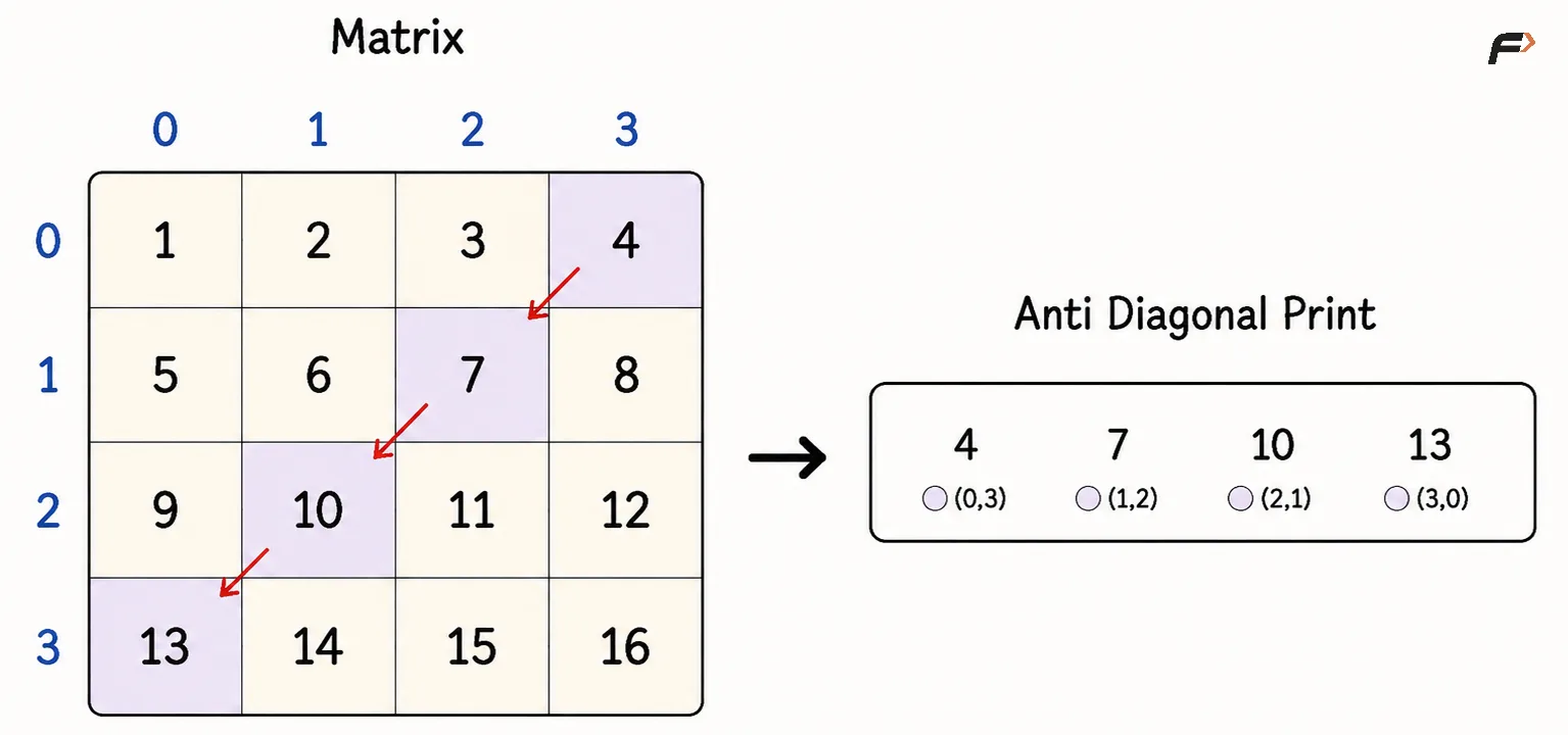
anti diagonal
Complexity Analysis
Time Complexity: O(min(N, M)), one anti-diagonal cell is visited for every valid row-column pair.
Space Complexity: O(1), only loop variables are used apart from output handling.
Interview follow-up Questions
An M × N matrix has M + N − 1 diagonals and M + N − 1 anti-diagonals. However, only one of each is the principal (main) diagonal and the secondary (anti-) diagonal.
Be the first to add a comment.